Horizontal Federated Learning case: Lymphoma detection

In this notebook we present a case where various hospitals want to identify cancerous tissue on lymph node section images. They have various hospitals that can train an AI model to detect if the tissue dected is cancerous or not.

This problem belongs to the Horizontal Federated Learning setting, since data sets will have the same feature space (same resolution of images) but differ in samples (different images).

With the help of Sherpa.ai Federated Learning framework, we design a solution to allow to train the AI model using the data sets of all hospitals without sharing any privacy-protected data or images, creating an AI model capable of detecting dangerous health conditions such as tumors while complying with privacy regulations. The architecture of the solution is:

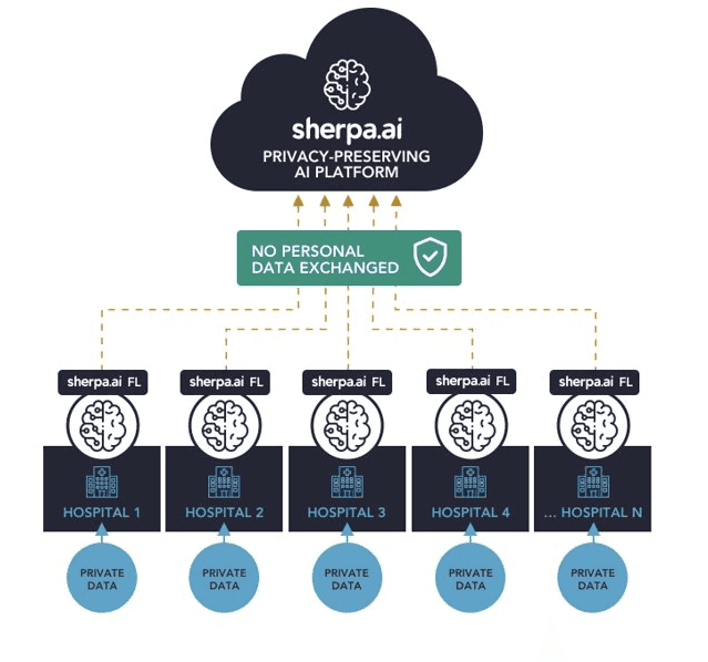
To set up the federated learning experiment we will show the simple steps for loading the dataset and distribute it to a federated network of clients, and we will define the model that will be trained in the federated learning rounds. In this notebook we are applying transfer learning as we are using the VGG16 model trained with the Imagenet dataset and personalization layer to use the knowledge of these model for our specific task.

Moreover, we will compare a local node's execution with only it's own data, the hipothetical case where all the data is centralized and the federated scenario to check the obtained models' performances against the testing data. Finally, we will further discuss the viability of horizontal Federated Learning.

The experiment's full dataset is really heavy, so for the viability of the execution variables need to be deleted, as a PC with 32 Gigabyte of RAM is not enough. In our case, a swapfile of 32 extra Gigabytes is used, however the process of training is slower.

Once that we have a general overview of our problem, the procedure is the following:

Index

1) Libraries and data

We are going to apply Horizontal Federated Learning to the dataset: PatchCamelyon (PCam). In order to realize this experiment, we need to obtain the dataset and then begin with the execution of the notebook.

Firstly, we load the libraries:

import os
import h5py
%matplotlib inline
import shfl
import tensorflow as tf
from shfl.auxiliar_functions_for_notebooks.functionsFL import *
from shfl.private.reproducibility import Reproducibility
from shfl.data_base.data_base import WrapLabeledDatabase
from keras.applications.vgg16 import VGG16
from keras import Input
from tensorflow.keras import layers, models

plt.style.use('seaborn')
np.random.seed(551)
Reproducibility(567)

2022-05-05 09:36:46.641814: W tensorflow/stream_executor/platform/default/dso_loader.cc:64] Could not load dynamic library 'libcudart.so.11.0'; dlerror: libcudart.so.11.0: cannot open shared object file: No such file or directory
2022-05-05 09:36:46.641835: I tensorflow/stream_executor/cuda/cudart_stub.cc:29] Ignore above cudart dlerror if you do not have a GPU set up on your machine.





<shfl.private.reproducibility.Reproducibility at 0x7fdcbd7e0790>

Let us firstly define a function to load the dataset from the downloaded files:

def load_dataset(path, mode):

    assert mode in ['train', 'valid', 'test']
    base_name = "camelyonpatch_level_2_split_{}_{}.h5"

    h5X = h5py.File(os.path.join(path, base_name.format(mode, 'x')), 'r')
    h5y = h5py.File(os.path.join(path, base_name.format(mode, 'y')), 'r')

    X = np.array(h5X.get('x'))
    Y = np.array(h5y.get('y'))

    return X, Y

Now that we have data and the function, let's extract the train and test data and divide it accordingly to some variables.

#train
path = "/home/x.sarrionaindia/Documentos/lymphoma/Datasets/PatchCamelyon/"
mode = 'train'
trainX, trainY = load_dataset(path, mode)

#test
path = "/home/x.sarrionaindia/Documentos/lymphoma/Datasets/PatchCamelyon/"
mode = 'test'
testX, testY = load_dataset(path, mode)

But first let's take a look to the images of the dataset:

from matplotlib import pyplot as plt

fig, axes = plt.subplots(3,5, figsize=(15,8))
for i,ax in enumerate(axes.flat):
    ax.imshow(trainX[i])

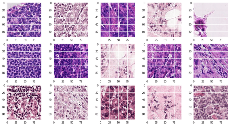
The images are fine, but in order to use them in a model in a proficiente way, there is the need of reshaping the data a little bit.

1.1) Necessary data transformations

The data comes without any preprocessing, so it is important that we apply transformations so that the model can digest it. First of all, we need to reformat the shape of the training data:

trainY_res = np.reshape(trainY,-1)
del trainY
trainY_res=np.eye(2)[trainY_res]

After that, we are going to wrap the data in the WrapLabeledDatabase class to convert it into federated data, and then divide it into the nodes.

database=WrapLabeledDatabase(trainX,trainY_res)

In this case, we could use local testing data to measure local performances. However, we are going to use a global test to compare it with the centralized case as the testing dataset is already defined for this experiment (the separate file we loaded earlier).

Now we adjust the data in a way that fits our data structure:

_, _, _, _ = database.load_data(train_proportion=1)

For this experiment, we are using 30 nodes simulating various hospitals, each of them containing a 5% of the existing data. Since we are using transfer learning, few samples are really needed to obtain a good performance with a model like that, so even though we used less data, the performance would still be good. In this case, the dataset has a lot of samples, so the 5% of the data is still a big proportion of the experiment.

besides, the sampling method gets randomly and evenly distributed data, so it divides it in a balanced way.

iid_distribution = shfl.data_distribution.IidDataDistribution(database)
nodes_federation, _, _ = iid_distribution.get_nodes_federation(num_nodes=30, percent=5)

As the data contained by the nodes is heavy, we need to delete unused variables to make this experiment lighter.

del iid_distribution
del database

After that, we need to apply remaining data transformations. Now that data is distributed in a format that the model can use, let's implement data normalization to improve model's results and performances. We took a small sample to calculate the mean and standard deviations as calculating the same values with the whole dataset is not really affecting the final results.

mean = np.mean(trainX[0:2000])

std = np.std(trainX[0:2000])

nodes_federation.apply_data_transformation(normalize_data, mean=mean, std=std);

del trainX

We also make the same operations for the testing dataset, and we keep it for later usage.

testY_res = np.reshape(testY,-1)
testY_res = np.eye(2)[testY_res]

testX_res = (testX - mean) / std

For saving memory, let's delete the remaining unused variables:

del testX
del testY

2) The model

Now, we need to define the model that will be used for the training. As specified before, we are going to use the VGG16 model that provides tensorflow. After obtaining it, we need to adjust some parameters (such as inputs and ouputs) to adapt it to our problem.

def model_builder(epoch_number):

    #Input configuration
    new_input = Input(shape=(96, 96, 3))

    #MobileNet configuration
    base_model = VGG16(input_tensor=new_input, classes=1,include_top=False)
    base_model.trainable = False
    

    #Personalization layer configuration
    flatten_layer = layers.Flatten()
    dense_layer_1 = layers.Dense(256, activation='relu') #256
    dense_layer_2 = layers.Dense(64, activation='relu') #64
    prediction_layer = layers.Dense(2, activation='softmax')

    #Model
    model = models.Sequential([
        base_model,
        flatten_layer,
        dense_layer_1,
        dense_layer_2,
        prediction_layer
    ])

    loss = tf.keras.losses.CategoricalCrossentropy()
    optimizer = tf.keras.optimizers.Adam()
    metrics = [tf.keras.metrics.categorical_accuracy]
    epochs = epoch_number
    batch_size = 32

    return shfl.model.DeepLearningModel(model=model, loss=loss, optimizer=optimizer,
                                        batch_size=batch_size, epochs=epochs, metrics=metrics)

3) Running the experiments

Now that the model is defined, we are going to set up all the possible experiments and make comparisons between them in a fairly realistic scenario.

3.1) Run the federated learning experiment

We create the components for the federated learning experiment and we assemble everything into the federated government:

aggregator = shfl.federated_aggregator.FedAvgAggregator()
federated_government = shfl.federated_government.FederatedGovernment(model_builder(1), nodes_federation, aggregator)

2022-05-05 09:37:06.966039: W tensorflow/stream_executor/platform/default/dso_loader.cc:64] Could not load dynamic library 'libcuda.so.1'; dlerror: libcuda.so.1: cannot open shared object file: No such file or directory
2022-05-05 09:37:06.966061: W tensorflow/stream_executor/cuda/cuda_driver.cc:269] failed call to cuInit: UNKNOWN ERROR (303)
2022-05-05 09:37:06.966077: I tensorflow/stream_executor/cuda/cuda_diagnostics.cc:156] kernel driver does not appear to be running on this host (SH-083-WS): /proc/driver/nvidia/version does not exist
2022-05-05 09:37:06.966224: I tensorflow/core/platform/cpu_feature_guard.cc:151] This TensorFlow binary is optimized with oneAPI Deep Neural Network Library (oneDNN) to use the following CPU instructions in performance-critical operations:  AVX2 FMA
To enable them in other operations, rebuild TensorFlow with the appropriate compiler flags.

Now let's run the federated training:

federated_government.run_rounds(5, testX_res, testY_res, eval_freq=1) #1000 - 250

WARNING:tensorflow:5 out of the last 13 calls to <function Model.make_test_function.<locals>.test_function at 0x7fdba65f7a60> triggered tf.function retracing. Tracing is expensive and the excessive number of tracings could be due to (1) creating @tf.function repeatedly in a loop, (2) passing tensors with different shapes, (3) passing Python objects instead of tensors. For (1), please define your @tf.function outside of the loop. For (2), @tf.function has experimental_relax_shapes=True option that relaxes argument shapes that can avoid unnecessary retracing. For (3), please refer to https://www.tensorflow.org/guide/function#controlling_retracing and https://www.tensorflow.org/api_docs/python/tf/function for  more details.
WARNING:tensorflow:5 out of the last 13 calls to <function Model.make_test_function.<locals>.test_function at 0x7fdba6e979d0> triggered tf.function retracing. Tracing is expensive and the excessive number of tracings could be due to (1) creating @tf.function repeatedly in a loop, (2) passing tensors with different shapes, (3) passing Python objects instead of tensors. For (1), please define your @tf.function outside of the loop. For (2), @tf.function has experimental_relax_shapes=True option that relaxes argument shapes that can avoid unnecessary retracing. For (3), please refer to https://www.tensorflow.org/guide/function#controlling_retracing and https://www.tensorflow.org/api_docs/python/tf/function for  more details.
Evaluation in round 0:


2022-05-05 09:40:56.595529: W tensorflow/core/framework/cpu_allocator_impl.cc:82] Allocation of 3623878656 exceeds 10% of free system memory.



Collaborative model test -> loss: 0.515089750289917  categorical_accuracy: 0.741729736328125  

Evaluation in round 1:


2022-05-05 09:52:38.782069: W tensorflow/core/framework/cpu_allocator_impl.cc:82] Allocation of 3623878656 exceeds 10% of free system memory.



Collaborative model test -> loss: 0.4616725742816925  categorical_accuracy: 0.788055419921875  

Evaluation in round 2:


2022-05-05 10:05:16.886851: W tensorflow/core/framework/cpu_allocator_impl.cc:82] Allocation of 3623878656 exceeds 10% of free system memory.



Collaborative model test -> loss: 0.42378923296928406  categorical_accuracy: 0.8031005859375  

Evaluation in round 3:


2022-05-05 10:18:41.385404: W tensorflow/core/framework/cpu_allocator_impl.cc:82] Allocation of 3623878656 exceeds 10% of free system memory.



Collaborative model test -> loss: 0.42609497904777527  categorical_accuracy: 0.79974365234375  

Evaluation in round 4:


2022-05-05 10:30:33.879652: W tensorflow/core/framework/cpu_allocator_impl.cc:82] Allocation of 3623878656 exceeds 10% of free system memory.



Collaborative model test -> loss: 0.42271074652671814  categorical_accuracy: 0.80322265625  

Let's see the performance of the other metrics of the model. First we extract the model and we perform predictions.

federated_model = federated_government._server._model
predictions_fed = federated_model.predict(testX_res)

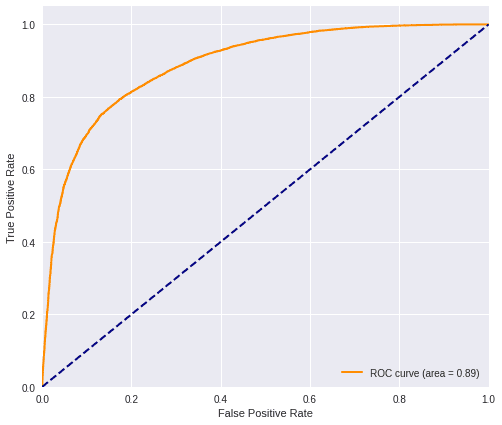
Then we calculate the ROC AUC and F1-Score values.

plot_roc(predictions_fed, testY_res)

fed_f1 = f1(testY_res, predictions_fed)
print('F1 score=', fed_f1)

F1 score= 0.7974747157484766

3.2) Run the experiment with only local data from a node

For the local test, we implemented a method to obtain the node's data experimentally. However, THIS IS NOT APPLICABLE IN A REAL CASE OR IN THE PLATFORM AND IT IS MADE FOR TESTING PURPOSES ONLY. All of these notebooks are made with an experimental implementation of the code where security measures are bypassed for explainability reasons. We take, for example, the data of the first node the local benchmark.

We extract the data from single node belonging to the federation.

local_model = model_builder(5)
identifier = federated_government._nodes_federation._data_nodes[0]._nodes_federation_identifier
data = federated_government._nodes_federation._data_nodes[0]._private_data[identifier]

We assign the same model to train only with local data.

local_model.train(data._data, data._label)
local_model.evaluate(testX_res, testY_res)

[('loss', 0.5594944953918457), ('categorical_accuracy', 0.772308349609375)]

Then, the resultant model will perform the predictions on it's own.

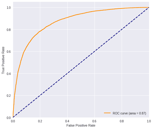
predictions_loc = local_model.predict(testX_res)

And we calculate the ROC AUC and the F1-Score values.

plot_roc(predictions_loc, testY_res)

loc_f1 = f1(testY_res, predictions_loc)
print('F1 score=', loc_f1)

F1 score= 0.7438459161602636

Then we delete remaining values that are unused in the future.

del local_model
del identifier
del data

3.3) Run the experiment with the data centralized

This correspond to the case of Traditional Machine Learning which requires all the data to be gathered in one single place. In practice, this is often forbidden by privacy regulations. The centralized data represents a node that has the whole dataset. In principle, this will imply a better accuracy but, for sure, this can not happen in a real world scenario, where the data are dispersed over different organizations under the protection of privacy restrictions. We will load the centralized data, joining the two datasets.

For the need to save memory, we are loading again the data from the nodes as we did in the local, as it is already ready for the training without further preprocessing.

trainX = []
trainY = []
for i in range(len(federated_government._nodes_federation._data_nodes)):
    identifier = federated_government._nodes_federation._data_nodes[i]._nodes_federation_identifier
    trainX=np.append(trainX,federated_government._nodes_federation._data_nodes[i]._private_data[identifier].data)
    trainY=np.append(trainY,federated_government._nodes_federation._data_nodes[i]._private_data[identifier].label)

del federated_government

Then we apply some transformations to the data and the labels to be able to feed them to the centralized model.

trainX=trainX.reshape(-1,96,96,3)

trainY = trainY.reshape(-1,2)

centralized_model = model_builder(5)

centralized_model.train(trainX, trainY)

centralized_model.evaluate(testX_res, testY_res)

[('loss', 0.49255627393722534), ('categorical_accuracy', 0.807647705078125)]

Then, the resultant model will perform the predictions on it's own.

predictions_cent = centralized_model.predict(testX_res)

We also delete the remaining variables to speedup the process.

del centralized_model
del testX_res

And we calculate the ROC AUC and the F1-Score values.

plot_roc(predictions_cent, testY_res)

cent_f1 = f1(testY_res, predictions_cent)
print('F1 score=', cent_f1)

F1 score= 0.8064605275278657

4) General comparison

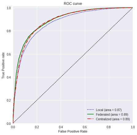
We are going now to use the ROC curve and the F1-Score to compare the different results that we have obtained. We will then be able to understand the improvements that using federated learning brings in this scenario.

4.1) ROC curve

We gather the different values used in each of the sections.

values=[predictions_loc, predictions_fed, predictions_cent]
titles=['Local', 'Federated', 'Centralized']
colors=['blue', 'green', 'red']
linestyle=[':','-','-.']

With the next function, we will plot a comparison between the metric of the three cases that we have presented:

plot_all_roc_curves(testY_res, values, titles, colors, linestyle)

4.2) F1-Score

Now we will show the F1-score metric of the three cases that we have presented:

values=[round(loc_f1, 3),
        round(fed_f1, 3),
        round(cent_f1, 3)]

titles=['Local',
        'Federated',
        'Centralized']

colors=['blue',
        'green',
        'red']

plot_all_metric(values, "F1-Score", titles, colors)

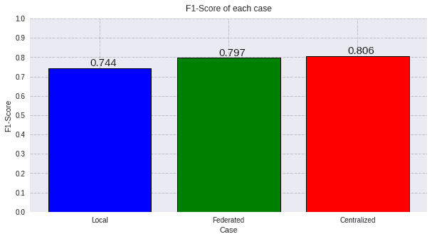
Taking into account the results of the ROC AUC and the F1-Score, we can assure that using a Federated Learning scenario in this problem is really convenient, since using transfer learning improves greatly the accuracy with few samples and the federated learning improves even more these metrics achieving a similar result to that of the centralized case.

Besides, in cases like this where the information could be really sensitive, it allows to collaborate with other entities without sharing any sensitive data. Bearing in mind the fact that the centralized case is forbidden by privacy regulations, federated learning is a really powerful tool to work with data silos preserving the privacy, both in performance and privacy terms.