Differential privacy: subsampling methods
In this notebook, we cover the concept of privacy augmentation by subsampling. That is, if a random sample is accessed instead of accessing the whole database, we can reduce the epsilon-delta cost of the access mechanism. We recommend taking a quick look at the paper Privacy Amplification by Subsampling: Tight Analyses via Couplings and Divergences.
Index
1) Composition & subsampling with the Laplace mechanism
On the one hand, we can dynamically query our private database until the privacy budget is completely spent and, on the other hand, we can increase the number of queries by applying them on a random subsample of the database. First of all, we define the composition experiment:
from shfl.private.node import DataNode
from shfl.differential_privacy.composition import AdaptiveDifferentialPrivacy
from shfl.differential_privacy.composition import ExceededPrivacyBudgetError
from shfl.differential_privacy.mechanism import LaplaceMechanism
import numpy as np
import matplotlib.pyplot as plt


def run_adaptive_comp_experiment(global_eps_delta, eps_delta_access):
    # Size of the data stored
    data_size = 100

    # Define a place to store the data
    node_single = DataNode()

    # Store the private data
    node_single.set_private_data(name="secret", data=np.ones(data_size))

    # Choose your favorite differentially_private_mechanism
    dpm = LaplaceMechanism(sensitivity=1, epsilon=eps_delta_access)

    # Here we are specifying that we want to use composition theorems for Privacy Filters
    # DP mechanism
    default_data_access = AdaptiveDifferentialPrivacy(global_eps_delta, mechanism=dpm)
    node_single.configure_data_access("secret", default_data_access)

    result_query = []
    while True:
        try:
            # Queries are performed using the Laplace mechanism
            result_query.append(node_single.query(private_property="secret"))
        except ExceededPrivacyBudgetError:
            # At this point we have spent the entire privacy budget
            break

    return result_query
Now, we specify the privacy budget and epsilon values for our experiment.
global_epsilon_delta = (2e-1, 2e-30)
epsilon_values = np.arange(2e-3, 2e-1, 2e-3)
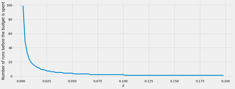
Finally, we plot the experiment results:
plt.style.use('fivethirtyeight')

fig, ax = plt.subplots(nrows=1, ncols=1, figsize=(16,6))
y_axis=[len(run_adaptive_comp_experiment(global_epsilon_delta, e)) for e in epsilon_values]
ax.plot(epsilon_values, y_axis)
ax.set_xlabel('$\epsilon$')
ax.set_ylabel('Number of runs before the budget is spent')

plt.show()
2022-03-23 09:11:17.855493: W tensorflow/stream_executor/platform/default/dso_loader.cc:64] Could not load dynamic library 'libcudart.so.11.0'; dlerror: libcudart.so.11.0: cannot open shared object file: No such file or directory
2022-03-23 09:11:17.855509: I tensorflow/stream_executor/cuda/cudart_stub.cc:29] Ignore above cudart dlerror if you do not have a GPU set up on your machine.

2) Including subsampling to the experiment
If we access the private data of size with a ()-differentially private mechanism over a random subsample without replacement of size , then the mechanism is ()-differentially private with:
Let's see what happens when we modify the experiment to introduce random subsampling:
from shfl.differential_privacy.privacy_amplification_subsampling import SampleWithoutReplacement

def run_adaptive_comp_experiment_sampling_without_replacement(global_eps_delta, eps_delta_access, data_size, sample_size):
    # Define a place to store the data
    node_single = DataNode()

    # Store the private data
    node_single.set_private_data(name="secret", data=np.ones(data_size))

    # Choouse your favourite differentially_private_mechanism
    dpm = LaplaceMechanism(sensitivity=1, epsilon=eps_delta_access)

    # Use a sampling method
    sampling_method = SampleWithoutReplacement(dpm, sample_size, data_size)

    # Here we are specifing that we want to use composition theorems for Privacy Filters
    # dp-mechanis
    default_data_access = AdaptiveDifferentialPrivacy(global_eps_delta, mechanism=sampling_method)
    node_single.configure_data_access("secret", default_data_access)

    result_query = []
    while True:
        try:
            # Queries are performed using the Laplace mechanism
            result_query.append(node_single.query(private_property="secret"))
        except ExceededPrivacyBudgetError:
            # At this point we have spent all our privacy budget
            break

    return result_query
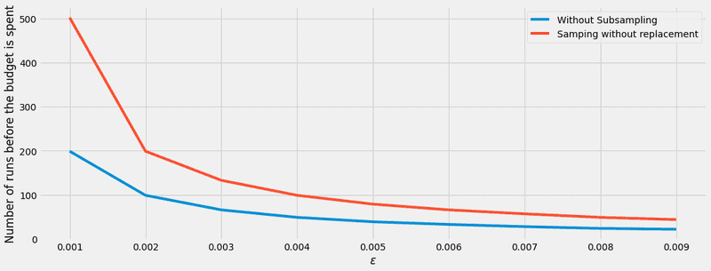
Now we plot both experiments to see the comparison between them:
global_epsilon_delta = (2e-1, 2e-30)
epsilon_values = np.arange(1e-3, 1e-2, 1e-3)
data_size = (100,)
sample_size = 50
plt.style.use('fivethirtyeight')

fig, ax = plt.subplots(nrows=1, ncols=1, figsize=(16,6))
y_axis=[len(run_adaptive_comp_experiment(global_epsilon_delta, e)) for e in epsilon_values]
ax.plot(epsilon_values, y_axis, label="Without Subsampling")

y_axis=[len(run_adaptive_comp_experiment_sampling_without_replacement(global_epsilon_delta, e, data_size, sample_size)) for e in epsilon_values]
ax.plot(epsilon_values, y_axis, label="Samping without replacement")

ax.set_xlabel('$\epsilon$')
ax.set_ylabel('Number of runs before the budget is spent')

plt.legend(title = "", loc="upper right")
plt.show()

We clearly see thath the subsampling method increases the number of queries needed to spend the privacy budget. But, how does the size of the sample modify these results?
3) Varying the sample size in the subsampling method
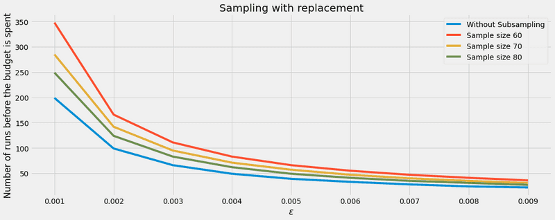
Let's see what happens with the subsampling when we change the sample size. For this purpose, we repeat the same experiment with different sample sizes:
global_epsilon_delta = (2e-1, 2e-30)
epsilon_values = np.arange(1e-3, 1e-2, 1e-3)
data_size = (100,)
samples_size = [60, 70, 80]
plt.style.use('fivethirtyeight')

fig, ax = plt.subplots(nrows=1, ncols=1, figsize=(16,6))


y_axis=[len(run_adaptive_comp_experiment(global_epsilon_delta, e)) for e in epsilon_values]
ax.plot(epsilon_values, y_axis, label="Without Subsampling")

for s_size in samples_size:
    y_axis_0=[len(run_adaptive_comp_experiment_sampling_without_replacement(global_epsilon_delta, e, data_size, s_size)) for e in epsilon_values]
    ax.plot(epsilon_values, y_axis_0, label="Sample size {}".format(s_size))

ax.set_xlabel('$\epsilon$')
ax.set_ylabel('Number of runs before the budget is spent')
ax.set_title('Sampling with replacement')
ax.legend(title = "", loc="upper right")

plt.show()

So, we can conclude that even with a relatively big sample (80% of the total size), the improvement over the non-sampling scheme is still great. Particularly, the improvement is grealy noticeable when , which makes the Gaussian Mechanism ideal, since to achieve ()-DP must be smaller than 1. That is, the Gaussian Mechanism and the subsampling methods, when applied together, can ensure a minor quantity of noise and a smaller privacy budget expenditure, at the cost of accessing a small random subsampling of the data.
4) Using subsampling methods in combination with the Gaussian mechanism
from shfl.differential_privacy.privacy_amplification_subsampling import SampleWithoutReplacement
from shfl.differential_privacy.mechanism import GaussianMechanism

def run_adaptive_comp_experiment(global_eps_delta, eps_delta_access):
    # Size of the data stored
    data_size = (100,)

    # Define a place to store the data
    node_single = DataNode()

    # Store the private data
    node_single.set_private_data(name="secret", data=np.ones(data_size))

    # Choose your favorite differentially_private_mechanism
    dpm = GaussianMechanism(sensitivity=1, epsilon_delta=eps_delta_access)

    # Here we are specifying that we want to use composition theorems for Privacy Filters
    # DP mechanism
    default_data_access = AdaptiveDifferentialPrivacy(global_eps_delta, mechanism=dpm)
    node_single.configure_data_access("secret", default_data_access)

    result_query = []
    while True:
        try:
            # Queries are performed using the Laplace mechanism
            result_query.append(node_single.query(private_property="secret"))
        except ExceededPrivacyBudgetError:
            # At this point we have spent the entiry privacy budget
            break

    return result_query

def run_adaptive_comp_experiment_sampling_without_replacement(global_eps_delta, eps_delta_access, data_size, sample_size):
    # Define a place to store the data
    node_single = DataNode()

    # Store the private data
    node_single.set_private_data(name="secret", data=np.ones(data_size))

    # Choose your favorite differentially_private_mechanism
    dpm = GaussianMechanism(sensitivity=1, epsilon_delta=eps_delta_access)

    # Use a sampling method
    sampling_method = SampleWithoutReplacement(dpm, sample_size, data_size)

    # Here we are specifying that we want to use composition theorems for Privacy Filters
    # DP mechanism
    default_data_access = AdaptiveDifferentialPrivacy(global_eps_delta, mechanism=sampling_method)
    node_single.configure_data_access("secret", default_data_access)

    result_query = []
    while True:
        try:
            # Queries are performed using the Laplace mechanism
            result_query.append(node_single.query(private_property="secret"))
        except ExceededPrivacyBudgetError:
            # At this point we have spent the entire privacy budget
            break

    return result_query
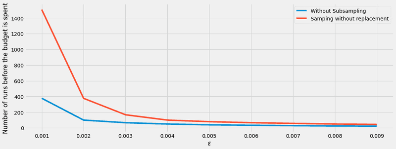
In order to make a similar comparison, we make the experiment without subsampling and the one with subsampling, using both the Gaussian mechanism. The results can be seen here below:
global_epsilon_delta = (2e-1, 2e-10)
epsilon_values = np.arange(1e-3, 1e-2, 1e-3)
delta_access = 2e-20
data_size = (100,)
sample_size = 50
plt.style.use('fivethirtyeight')

fig, ax = plt.subplots(nrows=1, ncols=1, figsize=(16,6))
y_axis=[len(run_adaptive_comp_experiment(global_epsilon_delta, (e, delta_access))) for e in epsilon_values]
ax.plot(epsilon_values, y_axis, label="Without Subsampling")

y_axis=[len(run_adaptive_comp_experiment_sampling_without_replacement(global_epsilon_delta, (e, delta_access), data_size, sample_size)) for e in epsilon_values]
ax.plot(epsilon_values, y_axis, label="Samping without replacement")

ax.set_xlabel('$\epsilon$')
ax.set_ylabel('Number of runs before the budget is spent')

plt.legend(title = "", loc="upper right")
plt.show()

It is clear that the queries needed to spend the privacy budget are much higher with very low values of . However, on higher values of the sampling without replacement makes little to no difference at all on the number of queries.