Basic Concepts of Vertical Federated Learning (assuming PSI*)
Federated Learning is a Machine Learning paradigm aimed at learning models from decentralized data, such as data located on users’ smartphones, in hospitals, or banks, and ensuring data privacy. This is achieved by training the model locally in each node (e.g., on each smartphone, at each hospital, or at each bank), sharing the model-updated local parameters (not the data) and securely aggregating them to build a better global model.
Traditional Machine Learning requires all the data to be gathered in one single place. In practice, this is often forbidden by privacy regulations. For this reason, Federated Learning is introduced with the goal is to learn from a large amount of data, while preserving privacy.
What is Vertical Federated Learning (VFL)?
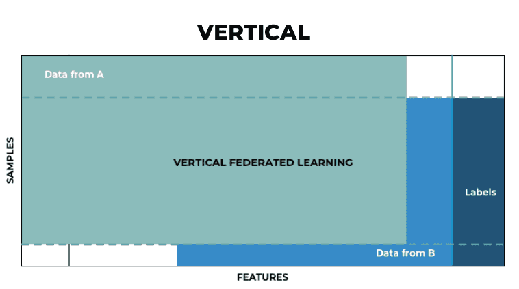
The sopported Federated Learning categories are: Horizontal, Vertical and Transfer. In this notebook we will focus on Vertical Federated Learning, where the nodes share overlapping samples (share the same sample ID space) but differ in data features. Feature/variables/attributes makes reference to a single property of the dataset, i.e, the columns. Sample makes reference to the instances/objects/records that contais the same structure as the dataset, i.e, the rows.
Vertical Federated Learning (VFL) is then the process of aggregating different features and computing the training loss and gradients in a privacy-preserving manner to build a model with data from both parties collaboratively. VFL employs this heterogeneity to train a more accurate model. The main idea to do this, is to split a Neural Network among different parties and a server. This will be described in 1.3.
(*) We will work only with the clients both parties have in common. This is assuming that the Private Set Intersection (PSI) protocol has already been applied.
The next figure shows the problem that we are going to solve:
In this notebook we will simulate a fictional scenario where a Bank and an Insurance Company want to collaborate to train a model using Sherpa.ai's platform in a private way that will allow to predict the likelihood of a bank's client to subscribe to a long-term deposit without compromising any data.
The general description of the problem is:
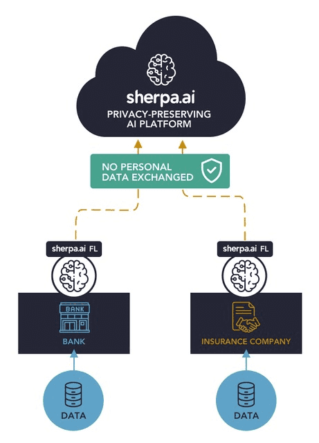
Using the the dataset Bank marketing campaigns dataset and in order to simulate a vertically partitioned training data, we will use some of the features as the data of one client (bank), and the rest for the other client (insurance).
Importance of the prediction of the output label:
A label (class label, output, prediction, target, or response) is the special attribute to be predicted based on all the input attributes.
A general description of the data:
Bank's data:
- 1 - age: Age of the lead (numeric)
- 2 - job: Type of job (categorical: "admin.","blue-collar","entrepreneur","housemaid","management","retired","self-employed","services","student","technician","unemployed","unknown")
- 3 - marital: Marital status (categorical: "divorced","married","single","unknown"; note: "divorced" means divorced or widowed)
- 4 - education (categorical: "basic.4y","basic.6y","basic.9y","high.school","illiterate","professional.course","university.degree","unknown")
- 5 - default: Does the lead have any default (unpaid) credit? (categorical: "no","yes","unknown")
- 6 - housing: Does the lead have any housing loan? (categorical: "no","yes","unknown")
- 7 - loan: Does the lead have any personal loan? (categorical: "no","yes","unknown")
- 8 - label - Has the client subscribed a term deposit? (binary: "yes","no")
Insurance's data:
- 9 - contact: Contact communication type (categorical: "cellular","telephone")
- 10 - month: Last contact month of year (categorical: "jan", "feb", "mar", …, "nov", "dec")
- 11 - dayofweek: Last contact day of the week (categorical: "mon","tue","wed","thu","fri")
- 12 - campaign: number of contacts performed during this campaign and for this client (numeric, includes last contact)
- 13 - pdays: Number of days that passed by after the client was last contacted from a previous campaign (numeric; 999 means client was not previously contacted)
- 14 - previous: Number of contacts performed before this campaign and for this client (numeric)
- 15 - poutcome: Outcome of the previous marketing campaign (categorical: "failure","nonexistent","success")
- 16 - emp.var.rate: employment variation rate - quarterly indicator (numeric)
- 17 - cons.price.idx: Consumer price index - monthly indicator (numeric)
- 18 - cons.conf.idx: Consumer confidence index - monthly indicator (numeric)
- 19 - euribor3m: Euribor 3 month rate - daily indicator (numeric)
- 20 - nr.employed: Number of employees - quarterly indicator (numeric)
We want both parties to have a prediction model to detect if a person will subscribe a term deposit (variable "y") based on these two datasets. A term deposit is a deposit account in a financial institution that is made for a specific period of time. These term deposits are usually made at banks or saving and loans. The depositors often prefer term deposits because they pay more interest than traditional savings accounts, yet are just as safe. Furthermore, banks are willing to pay more interest on a term deposit because they know the money will stay deposited for a fixed time period. **This helps them better manage their capital ratios, so maximizing the prediction is preponderant.
Once that we have a general overview of our problem, the procedure is the following:
Index
0) Libraries and data
First of all, we will load the libraries that we are going to use:
import pandas as pd
import numpy as np
import matplotlib.pyplot as plt
import warnings

from shfl.model.vertical_deep_learning_model_pt import VerticalNeuralNetServerModelPyTorch
from shfl.model.vertical_deep_learning_model_pt import VerticalNeuralNetClientModelPyTorch
from shfl.model.deep_learning_model_pt import DeepLearningModelPyTorch
from shfl.private.federated_operation import VerticalServerDataNode
from shfl.data_base.data_base import split_train_test
from shfl.federated_government.vertical_federated_government import VerticalFederatedGovernment
from shfl.federated_aggregator import FedSumAggregator
from shfl.private.data import LabeledData
from shfl.private.federated_operation import federate_list
from shfl.private.reproducibility import Reproducibility
from shfl.auxiliar_functions_for_notebooks.functionsFL import *
from shfl.auxiliar_functions_for_notebooks.preprocessing import preprocessing_data, label_encoder

plt.style.use('seaborn')
pd.set_option("display.max_rows", 30, "display.max_columns", None)
warnings.filterwarnings('ignore')
Reproducibility(567)
2022-04-25 11:49:03.654096: W tensorflow/stream_executor/platform/default/dso_loader.cc:64] Could not load dynamic library 'libcudart.so.11.0'; dlerror: libcudart.so.11.0: cannot open shared object file: No such file or directory
2022-04-25 11:49:03.654113: I tensorflow/stream_executor/cuda/cudart_stub.cc:29] Ignore above cudart dlerror if you do not have a GPU set up on your machine.
<shfl.private.reproducibility.Reproducibility at 0x7f85406634f0>We load the data of the bank and the insurance:
data_bank = pd.read_csv("./data_bank.csv", sep=",")
data_insurance = pd.read_csv("./data_insurance.csv", sep=",")
The clients' data are the one that we have already described, so we show the first rows of the data:
data_bank.head()| age | job | marital | education | default | housing | loan | label | |
|---|---|---|---|---|---|---|---|---|
| 0 | 35 | entrepreneur | married | basic.9y | no | yes | no | no |
| 1 | 36 | blue-collar | divorced | basic.9y | unknown | no | no | no |
| 2 | 40 | entrepreneur | married | university.degree | no | no | no | no |
| 3 | 42 | services | married | high.school | no | no | no | no |
| 4 | 25 | student | single | high.school | no | yes | yes | yes |
data_insurance.head()| campaign | pdays | previous | emp.var.rate | cons.price.idx | cons.conf.idx | euribor3m | nr.employed | contact | month | day_of_week | poutcome | |
|---|---|---|---|---|---|---|---|---|---|---|---|---|
| 0 | 1 | 999 | 0 | -1.7 | 94.027 | -38.3 | 0.890 | 4991.6 | telephone | aug | wed | nonexistent |
| 1 | 2 | 999 | 0 | 1.4 | 94.465 | -41.8 | 4.961 | 5228.1 | telephone | jun | thu | nonexistent |
| 2 | 1 | 999 | 0 | 1.4 | 93.918 | -42.7 | 4.963 | 5228.1 | cellular | jul | wed | nonexistent |
| 3 | 3 | 999 | 0 | 1.1 | 93.994 | -36.4 | 4.855 | 5191.0 | telephone | may | fri | nonexistent |
| 4 | 2 | 6 | 3 | -1.7 | 94.055 | -39.8 | 0.761 | 4991.6 | cellular | jun | tue | success |
And we explore how many instances and features each node has:
print('There are {} observations with {} features for the bank.'.format(data_bank.shape[0], data_bank.shape[1]))
print('There are {} observations with {} features for the insurance.'.format(data_insurance.shape[0], data_insurance.shape[1]))
There are 41188 observations with 8 features for the bank.
There are 41188 observations with 12 features for the insurance.We make sure that there are no missing rows (elements without data):
sum(np.sum(data_bank.isna()))0sum(np.sum(data_insurance.isna()))0We now convert the target ("yes" or "no") of the Bank into numeric to be able to make predictions:
labels_total_numeric = label_encoder(data_bank.label)And we split it from the dataset:
data_bank=data_bank.drop("label", axis=1)1) Prepare the data and the models for the vertical federated learning scenario preserving the privacy
1.1) Bank Data Preprocessing
We have to One Hot Encode the categorical variables and normalize the numeric variables:
data_bank_array = preprocessing_data(data_bank)We have already supposed that the labels are assigned to the bank. We split the data sets into training data and testing data.
train_data_bank, train_labels, test_data_bank, test_labels = split_train_test(data_bank_array,
                                                                              labels_total_numeric)
1.2) Insurance Data Preprocessing
We do the same preprocessing and splitting for the insurance:
data_insurance_array = preprocessing_data(data_insurance)train_data_ins, test_data_ins = split_train_test(data_insurance_array)1.3) Deploying the full neural network model
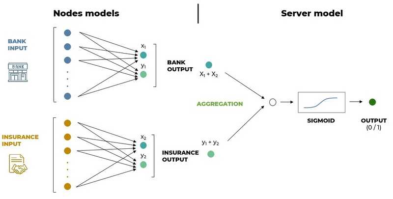
The scheme of the neural network that we are going to build to fulfil the vertical federated scenario is:
We will deploy two neural networks corresponding to two nodes in the federation, one for the bank and the other for the insurance company. The outputs of each neural network (embeddings), are aggregated by a sum through the server. This aggregation will be the input of the server while the output will be the prediction. The scheme of the neural network that we are going to build with PyTorch to fulfill the vertical federated scenario is the following:
Our goal in this notebook will be to prove that the federated model performs better than a model that would only be trained with data which the bank owns while also respecting all the privacy regulations. We will also compare our results with the predictions of a centralized (without privacy) model trained in the aggregated dataset that, of course, we expect to perform better without respecting any privacy regulations.
1.3.1) Create the federated nodes
We generate the federated nodes with the next function:
nodes_federation = federate_list([train_data_bank, train_data_ins],fed_data_node_type="HeterogeneousDataNode")And we will create the test data:
test_data = [test_data_bank, test_data_ins]We need to specify which model to use for each client node. As this is a classification problem, we will use a really simple one, a logistic regression. It can be modelled as a function that can take in any number of inputs and constrain the output to be between 0 and 1. This means, we can think of Logistic Regression as a one-layer neural network.
Bearing this in mind, the clients will run a neural network model, but of course they will have different input sizes since they possess different number of features. As we don't use hidden layers for the clients' model, these will result in linears models for both the bank and the insurance, as we have mentioned above.
client_out_dim = 2

model0 = nn.Sequential(
    nn.Linear(train_data_bank.shape[1], client_out_dim, bias=True),
)

model1 = nn.Sequential(
    nn.Linear(train_data_ins.shape[1], client_out_dim, bias=True),
)

optimizer0 = torch.optim.SGD(params=model0.parameters(), lr=0.001)
optimizer1 = torch.optim.SGD(params=model1.parameters(), lr=0.001)

batch_size = 32
model_nodes = [VerticalNeuralNetClientModelPyTorch(model=model0, loss=None, optimizer=optimizer0, batch_size=batch_size),
               VerticalNeuralNetClientModelPyTorch(model=model1, loss=None, optimizer=optimizer1, batch_size=batch_size)]
The variable client_out_dim is the tradeoff between the accuracy of the train model and the computational cost of the training. It is useful to think this as "the dimension of a hidden layer" that will receive the server.
1.3.2) Create the server model
In the Vertical FL, each node, including the server, is allowed to possess a different model and different methods for interacting with the clients.
The server is assigned a linear model, along with the data to train on. In this particular case, the Bank will be the server (because it has all the labels we want to predict) but also a client (node), because it has the data. Note that the distinction between client and server is only virtual and not necessarily physical, since a single node might be both client and server, allowing multiple roles for the same physical node.
# Define the model of the server node
model_server = torch.nn.Sequential(
    torch.nn.Linear(client_out_dim, 1, bias=True),
    torch.nn.Sigmoid())
loss_server = torch.nn.BCELoss(reduction="mean")
optimizer_server = torch.optim.SGD(params=model_server.parameters(), lr=0.001)

model = VerticalNeuralNetServerModelPyTorch(model_server, loss_server, optimizer_server,
                                      metrics={"accuracy":accuracy})

# Create the server node with the shfl platform
server_node = VerticalServerDataNode(
    nodes_federation=nodes_federation,
    model=model,
    aggregator=FedSumAggregator(),
    data=LabeledData(data=None, label=train_labels.reshape(-1,1).astype(np.float32)))

# Configure data access to nodes and server
nodes_federation.configure_model_access(meta_params_query)
server_node.configure_model_access(meta_params_query)
server_node.configure_data_access(train_set_evaluation)
Pytorch models expect by default input data to be float:
# Convert to float
nodes_federation.apply_data_transformation(cast_to_float);
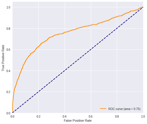
The metric that we are going to use is the AUC (Area Under Curve) of the ROC. The ROC (Receiver Operating Characteristic) Curve is a useful diagnostic tool for understanding the trade-off for different thresholds and the AUC provides a useful number for comparing models based on their general capabilities. It is equivalent to the probability that a randomly chosen positive instance is ranked higher than a randomly negative instance. In practice, the AUC performs well as a general measure of predictive accuracy.
2) Run the experiment
2.1) Federated
One last concept that has to be defined, is a round in federated learning: Each round of the process consists in transmitting the current global model state to participating nodes, training local models on these local nodes to produce a set of potential model updates at each node, and then aggregating and processing these local updates into a single global update and applying it to the global model.
We are ready to launch our federated experiment with 10000 communication rounds:
# Create federated government
federated_government = VerticalFederatedGovernment(model_nodes,
                                                   nodes_federation,
                                                   server_node=server_node)
# Run training and testing
federated_government.run_rounds(n_rounds=10001,
                                test_data=test_data,
                                test_label=test_labels.reshape(-1,1),
                                eval_freq=1000)
Evaluation in round 0 :
Loss: 0.9052186608314514 Accuracy: 0.10924981791697014
Evaluation in round 1000 :
Loss: 0.5681487321853638 Accuracy: 0.8153678077203205
Evaluation in round 2000 :
Loss: 0.36543920636177063 Accuracy: 0.8943918426802622
Evaluation in round 3000 :
Loss: 0.31213048100471497 Accuracy: 0.8959698956057296
Evaluation in round 4000 :
Loss: 0.298957884311676 Accuracy: 0.8994901675163874
Evaluation in round 5000 :
Loss: 0.294155091047287 Accuracy: 0.8996115562029618
Evaluation in round 6000 :
Loss: 0.29171422123908997 Accuracy: 0.9007040543821316
Evaluation in round 7000 :
Loss: 0.2902122735977173 Accuracy: 0.9011896091284293
Evaluation in round 8000 :
Loss: 0.28916528820991516 Accuracy: 0.9011896091284293
Evaluation in round 9000 :
Loss: 0.28827354311943054 Accuracy: 0.9014323865015781
Evaluation in round 10000 :
Loss: 0.2875165045261383 Accuracy: 0.9013109978150037As we can observe, after 10000 comunication rounds, the accuracy has improve up to 0.754.
If we plot the results of our federated experiment:
predictions_fed = federated_government._server.predict_collaborative_model(test_data)
plot_roc(predictions_fed, test_labels)
2.2) Local ( Data from the bank only )
The local case refers to the situation where we only have the data belonging to one of the clients, which in this case is the bank. This will be useful to understand how the insurance data improves the metric of the model obtained by using only the data of the bank.
With this said, we show the metric obtained if we only have the data from the bank:
sklearn_logistic_operation(train_data_bank, train_labels, test_data_bank, test_labels)
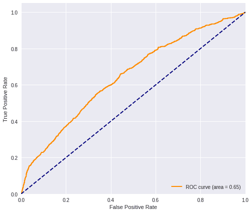
As to do a fair comparison we have to use the same models, we opt to create our own local model to compare with the federate scenario. In any case, we can do the logistic operation with Sklearn to check that works very similar to our model.
predictions_loc = logistic_operation(train_data_bank.shape[1], train_data_bank, train_labels,
                                      test_data_bank, test_labels)

2.3) Centralized ( Data joined without any privacy )
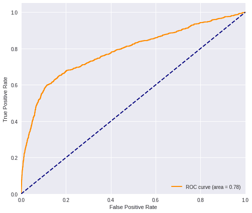
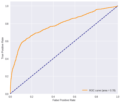
The centralized data represents a node that has the whole dataset, joined without any kind of privacy. In principle, this will imply a better accuracy but, for sure, this can not happen in a real world scenario, where the data are dispersed over different organizations under the protection of privacy restrictions. We will load the centralized data, joining the two datasets.
centralized_data = pd.read_csv("./centralized_data.csv", sep=",")We do the same preprocessing as with the local nodes.
centralized_data = preprocessing_data(centralized_data)And we split in train and test as we did with the local nodes:
train_centralized_data, test_centralized_data = split_train_test(centralized_data)The labels will be the same as the bank, this is, labels_total_numeric, since we have already supossed that the entity resolution is already done.
Now we show the metric with the data of the bank and the insurance aggregated in a way that the data privacy principle is not respected:
# Idem of local
sklearn_logistic_operation(train_centralized_data, train_labels, test_centralized_data, test_labels)
predictions_cent = logistic_operation(train_centralized_data.shape[1], train_centralized_data,
                                       train_labels, test_centralized_data, test_labels)
2.4) Comparison
2.4.1) ROC curve
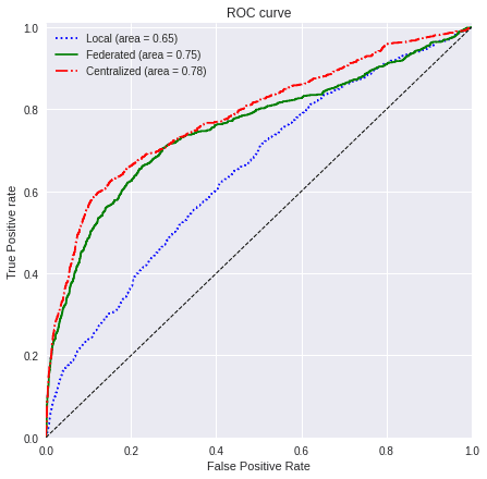
With the next function, we will plot a comparison between the metric of the three cases that we have presented:
values=[predictions_loc, predictions_fed, predictions_cent]
titles=['Local', 'Federated', 'Centralized']
colors=['blue', 'green', 'red']
linestyle=[':','-','-.']plot_all_roc_curves(test_labels, values, titles, colors, linestyle)
2.4.2) F1 Score
n_classes=2

values_f1_fed = (predictions_fed > 0.5).astype(int)

values_f1_loc = (predictions_loc > 0.5).astype(int)

values_f1_cent = (predictions_cent > 0.5).astype(int)


score_fed_f1 = f1_score(test_labels, values_f1_fed, average='macro')

score_loc_f1 = f1_score(test_labels, values_f1_loc, average='macro')

score_cent_f1 = f1_score(test_labels, values_f1_cent, average='macro')

values=[round(score_loc_f1, 3), round(score_fed_f1, 3), round(score_cent_f1, 3)]
titles=['Local', 'Federated', 'Centralized']
colors=['blue', 'green', 'red']
plot_all_metric(values, "F1-Score", titles, colors)
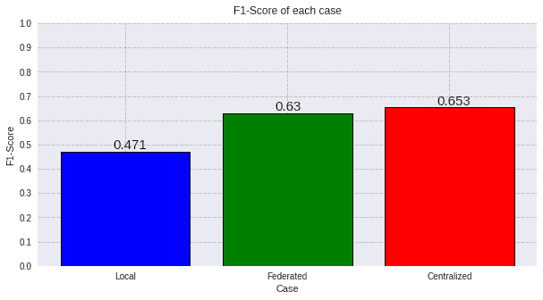
These figure show three different results:
- In , we have the result of using just the local data of the bank. This correspond to the local case, where we have the features of the bank but not the insurance.
- In , we have the result of the federate experiment, where we have used the features of both clients in a privacy preserving manner using Private Set Intersection.
- In , we have the result of using the centralized data aggregation of both clients without any kind of privacy.
The figures show the benefit of using the data of both clients in a privacy preserving manner in comparison with just one client. Even though the best scenario in term of the metric is where we use the data in a centralized way, the improvement with respect to the federated case is not really significant, since it is really similar (only 0.03 higher regarding the ROC AUC and 0.021 regarding the F1 score)
In summary, by using linear models in the nodes, the results of the ROC AUC for the three different cases are:
Local (0.65) << Federated (0.75) < Centralized (0.78)
We improve by 0.12 the prediction of the bank by using the data of the insurance in a federated way while preserving the privacy. By using all the data BUT without preserving the privacy, we would only improve a 0.02 with respect to the federated model.
And the results of the F1 score are:
Local (0.47) << Federated (0.63) < Centralized (0.65)
We improve by 0.16 the prediction of the bank by using the data of the insurance in the federated way. By using all the data BUT without preserving the privacy, we would only improve a 0.021 with respect to the federated model.
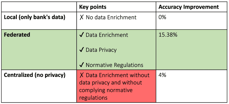
The model trained with the bank's data solely has no data enrichment, whereas the federated one enjoys data enrichment, data privacy and complies with all the normative regulations, apart from having a greater accuracy improvement.
As a conclusion of this notebook, we can notice the benefits of using the Sherpa.ai’s Privacy-Preserving platform in a Vertical Federated scenario. The prediction is almost as much accurate as traditional machine learning methods, but with the significant benefit of ensuring the privacy of data and regulatory compliance.