⚠

Please note that these tutorials refer to a deprecated version of the platform. The current version of the platform, which is not publicly available, has a more advanced architecture and provides a wider range of functionalities. These tutorials are only for illustrative purposes and showcase a limited number of the platform’s capabilities.

Federated models: logistic regression

Here, we explain how to set up a federated classification experiment using a Logistic Regression model. Results from the federated learning are compared to the (non-federated) centralized learning. Moreover, we also show how the addition of differential privacy affects the performance of the Federated model. In these examples, we will generate synthetic data for the classification task. In particular, we will start from a two-dimensional case, since with only two features, we are able to easily plot the samples and the decision boundaries computed by the classifier. After that, we will repeat the experiment by adding more features and classes to the synthetic database.

Index

1) The data
2) The model
3) Run the federated learning experiment
4) Add differential privacy

4.1) Sensitivity by sampling
4.2) Run the federated learning experiment with differential privacy
4.3) F1-score comparison

5) Case with more features and classes

5.1) Run the federated learning experiment
5.2) Comparison with centralized training
5.3) Run the federated learning experiment with differential privacy
5.4) F1-score comparison

1) The data

We generate the data using the make_classification function from scikit-learn:

import shfl
from shfl.data_base.data_base import WrapLabeledDatabase
from sklearn.datasets import make_classification
import numpy as np
from shfl.auxiliar_functions_for_notebooks.functionsFL import *
from shfl.private.reproducibility import Reproducibility

# Comment to turn off reproducibility:
Reproducibility(1234)

# Create database:
n_features = 2
n_classes = 3
n_samples = 10000
data, labels = make_classification(
    n_samples=n_samples, n_features=n_features, n_informative=2, 
    n_redundant=0, n_repeated=0, n_classes=n_classes, 
    n_clusters_per_class=1, weights=None, flip_y=0.1, class_sep=0.4, random_state=1234)
database = WrapLabeledDatabase(data, labels)

train_data, train_labels, test_data, test_labels = database.load_data()

print("Shape of training and test data: " + str(train_data.shape) + str(test_data.shape))
print("Shape of training and test labels: " + str(train_labels.shape) + str(test_labels.shape))
print(train_data[0,:])

2022-03-24 18:06:42.790233: W tensorflow/stream_executor/platform/default/dso_loader.cc:64] Could not load dynamic library 'libcudart.so.11.0'; dlerror: libcudart.so.11.0: cannot open shared object file: No such file or directory
2022-03-24 18:06:42.790251: I tensorflow/stream_executor/cuda/cudart_stub.cc:29] Ignore above cudart dlerror if you do not have a GPU set up on your machine.


Shape of training and test data: (8000, 2)(2000, 2)
Shape of training and test labels: (8000,)(2000,)
[-0.44710436  0.43652886]

As previously mentioned, in this two-feature case, it is beneficial to visualize the results. For that purpose, we will use the following function:

import matplotlib.pyplot as plt

def plot_2D_decision_boundary(model, data, labels, title=None):
    # Step size of the mesh. The smaller it is, better the quality
    h = .02 
    # Color map
    cmap = plt.cm.Set1
    
    # Plot the decision boundary. For that, we will assign a color to each
    x_min, x_max = data[:, 0].min() - 1, data[:, 0].max() + 1
    y_min, y_max = data[:, 1].min() - 1, data[:, 1].max() + 1
    xx, yy = np.meshgrid(np.arange(x_min, x_max, h), np.arange(y_min, y_max, h))
    
    # Obtain labels for each point in mesh. Use last trained model.
    Z = model.predict(np.c_[xx.ravel(), yy.ravel()])
    
    # Put the result into a color plot
    Z = Z.reshape(xx.shape)
    fig, ax = plt.subplots(figsize=(9,6))
    plt.clf()
    plt.imshow(Z, interpolation='nearest',
               extent=(xx.min(), xx.max(), yy.min(), yy.max()),
               cmap=cmap,
               alpha=0.6,
               aspect='auto', origin='lower')
    # Plot data:
    plt.scatter(data[:, 0], data[:, 1], c=labels, cmap=cmap, s=40, marker='o')
    
    plt.title(title, fontsize=18)
    plt.xlim(x_min, x_max)
    plt.ylim(y_min, y_max)
    plt.xlabel('Feature 1', fontsize=18)
    plt.ylabel('Feature 2', fontsize=18)
    plt.tick_params(labelsize=15)

2) The model

The Sherpa.ai Federated Learning and Differential Privacy Framework offers support for the Logistic Regression model from scikit-learn. The user must specify, in advance, the number of features and the target classes: the assumption for this Federated Logistic Regression example is that each client's data possesses at least one sample of each class. Otherwise, each node might train a different classification problem, and it would be problematic to _aggregate the global model. Setting a model's state parameter to warm_start:True tells the clients to restart the training from the Federated round update. To assess the performance, we compute the Balanced Accuracy and the Kohen Kappa scores (see metrics):

from sklearn.linear_model import LogisticRegression
from shfl.model.linear_classifier_model import LinearClassifierModel

# Define the model:
classes = np.unique(train_labels)
def model_builder():
    sk_model = LogisticRegression(warm_start=True, solver='lbfgs', multi_class='auto')
    model = LinearClassifierModel(n_features=n_features, classes=classes, model=sk_model)
    return model

We can train the model on centralized data (i.e. non-federated), which will be our reference model:

# Train model on centralized data for comparison:
model_centralized = LinearClassifierModel(n_features=n_features, classes=classes)
model_centralized.train(train_data, train_labels)
print('Centralized test performance: ' + str(model_centralized.evaluate(test_data, test_labels)))

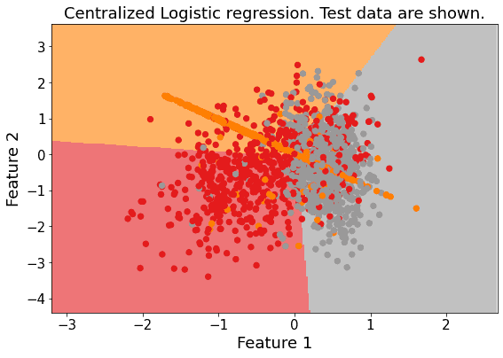
# Plot decision boundaries and test data for the centralized (non-Federated) case:
if n_features == 2:
    plot_2D_decision_boundary(model_centralized._model, 
                              test_data, test_labels, 
                              title = "Centralized Logistic regression. Test data are shown.")  
    
predictions_cent = model_centralized.predict(test_data)


Centralized test performance: [('balanced_accuracy', 0.6991963002582472), ('cohen_kappa', 0.5504229257243041)]

png

3) Run the federated learning experiment

We are ready to run our model in a federated configuration. We distribute the data over the nodes, assuming the data is IID. Next, we define the aggregation of the federated outputs to be the average of the client models.

# Distribute data over the nodes:
iid_distribution = shfl.data_distribution.IidDataDistribution(database)
n_clients = 5
nodes_federation, test_data, test_labels = iid_distribution.get_nodes_federation(num_nodes=n_clients, percent=100)
aggregator = shfl.federated_aggregator.FedAvgAggregator()


# Run the federated experiment:
federated_government = shfl.federated_government.FederatedGovernment(model_builder(), nodes_federation, aggregator)
federated_government.run_rounds(n_rounds=2, test_data=test_data, test_label=test_labels)

Evaluation in round 0:

Collaborative model test -> balanced_accuracy: 0.6986834797454265  cohen_kappa: 0.5496626604937622  

Evaluation in round 1:

Collaborative model test -> balanced_accuracy: 0.6986834797454265  cohen_kappa: 0.5496626604937622

It can be observed that the performance of the federated global model is generally superior with respect to the performance of each node, thus, the federated learning approach proves to be beneficial. Moreover, since no or little performance difference is observed between the federated rounds, we can conclude that the classification problem converges very early, in this setting, and no further rounds are required. This might be due to the IID nature of the client data when performing classification: each node gets a representative chunk of data and thus the local models are similar.

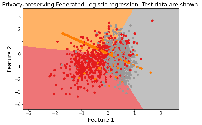
It can be observed that the performance of federated global model is comparable to the performance of the model trained on centralized data, and it produces similar decision boundaries.

# Plot decision boundaries and test data for the Federated case:
if n_features == 2:
    plot_2D_decision_boundary(federated_government._server._model, 
                              test_data, test_labels, 
                              title = "Federated Logistic regression. Test data are shown.")

png

4) Add differential privacy

We want to assess the impact of differential privacy (see The Algorithmic Foundations of Differential Privacy, Section 3.3) on the federated model's performance.

4.1) Model's sensitivity

In particular, we will use the Laplace mechanism. The noise added has to be of the same order as the sensitivity of the model's output, i.e., the model parameters of our logistic regression. In general, the sensitivity of a Machine Learning model is difficult to compute (for the Logistic Regression case, refer to Privacy-preserving logistic regression). An alternative strategy may be to estimate the sensitivity through a sampling procedure (e.g., see Rubinstein 2017. However, be advised that this would guarantee the weaker property of random differential privacy. This approach is convenient, since it allows for the sensitivity estimation of an arbitrary model or a black-box computer function. The Sherpa.ai Federated Learning and Differential Privacy Framework provides this functionality in the class SensitivitySampler.

We need to specify a distribution of the data to sample from. Generally, this requires previous knowledge and/or model assumptions. In order not to make any specific assumptions about the distribution of the dataset, we can choose a uniform distribution. We define our class of ProbabilityDistribution that uniformly samples over a data-frame. We could sample using the training data. However, since in a real case, the training data would be the actual client data, we wouldn't have access to it. Thus, we generate another synthetic dataset for sampling (in a real case, this could be a public database we are able to access):

class UniformDistribution(shfl.differential_privacy.ProbabilityDistribution):
    """
    Implement Uniform sampling over the data
    """
    def __init__(self, sample_data):
        self._sample_data = sample_data

    def sample(self, sample_size):
        row_indices = np.random.randint(low=0, high=self._sample_data.shape[0], size=sample_size, dtype='l')
        
        return self._sample_data[row_indices, :]
    
# Create sampling database:
n_samples = 150
sampling_data, sampling_labels = make_classification(
    n_samples=n_samples, n_features=n_features, n_informative=2, 
    n_redundant=0, n_repeated=0, n_classes=n_classes, 
    n_clusters_per_class=1, weights=None, flip_y=0.1, class_sep=0.1)    
sample_data = np.hstack((sampling_data, sampling_labels.reshape(-1,1)))

The class SensitivitySampler implements the sampling, given a query (i.e., the learning model itself, in this case). We only need to add the __call__ method to our model to make the object callable: it simply trains the model on the input data and outputs the trained parameters. We choose the sensitivity norm to be the $L_1$ norm and we apply the sampling. Typically, the value of the sensitivity is influenced by the size of the sampled data: the higher, the more accurate the sensitivity. Note that the sampling could be quite costly, since the query (i.e. the model, in this case) is called, each time.

from shfl.differential_privacy import SensitivitySampler
from shfl.differential_privacy import L1SensitivityNorm

class LogisticRegressionSample(LinearClassifierModel):
    
    def __call__(self, data_array):
        data = data_array[:, 0:-1]
        labels = data_array[:, -1]
        train_model = self.train(data, labels)
      
        return self.get_model_params()

distribution = UniformDistribution(sample_data)
sampler = SensitivitySampler()

n_data_size = 200
max_sensitivity, mean_sensitivity = sampler.sample_sensitivity(
    LogisticRegressionSample(n_features=n_features, classes=classes), 
    L1SensitivityNorm(), distribution, n_data_size=n_data_size, gamma=0.05)
print("Max sensitivity from sampling: " + str(max_sensitivity))
print("Mean sensitivity from sampling: " + str(mean_sensitivity))

Max sensitivity from sampling: [0.0924162176816866, 0.34331071747749325]
Mean sensitivity from sampling: [0.025176442836931993, 0.06353797841625748]

4.2) Run the federated learning experiment with differential privacy

Once the model's estimated sensitivity has been obtained, we fix the $\epsilon$ privacy budget and we can run the privacy-preserving Federated experiment

from shfl.differential_privacy import LaplaceMechanism

params_access_definition = LaplaceMechanism(sensitivity=max_sensitivity, epsilon=0.5)
nodes_federation.configure_model_params_access(params_access_definition)

federated_governmentDP = shfl.federated_government.FederatedGovernment(
    model_builder(), nodes_federation, aggregator)

federated_governmentDP.run_rounds(n_rounds=2, test_data=test_data, test_label=test_labels)

Evaluation in round 0:

Collaborative model test -> balanced_accuracy: 0.5541075345500124  cohen_kappa: 0.33085685501224893  

Evaluation in round 1:

Collaborative model test -> balanced_accuracy: 0.6746512447729263  cohen_kappa: 0.5126921543436849

As you might expect, the addition of random noise slightly alters the solution, but the model is still comparable to the non-private federated case:

# Plot decision boundaries and test data for Privacy-preserving Federated case:
if n_features == 2:
    plot_2D_decision_boundary(federated_governmentDP._server._model, test_data, test_labels,
                              title = "Privacy-preserving Federated Logistic regression. Test data are shown.")

png

Note 1: In this case, we only run a few federated rounds. However, in general, you should make sure not to exceed a fixed privacy budget.

Note 2: It is worth mentioning that the above results cannot be considered general. Some factors that considerably influence the classification problem are, for example, the training dataset, the model type, and the differential privacy mechanism used. In fact, the classification problem itself depends on the training data (number of features, whether the classes are separable or not etc.). We strongly encourage users to play with the values for generating the database (such as n_features, n_classes, n_samples, class_sep ... see their meaning here), or try different classification datasets, since convergence and accuracy of local and global models can be strongly affected. Moreover, even without changing the dataset, by running the present experiment multiple times (you need to comment the Reproducibility command line code), it is observed that the federated global model may also exhibit slightly better performance, when compared to the centralized model (we use random_state input, in order to always produce the same dataset). Similarly, the privacy-preserving federate model might exhibit even better performance, compared to the non-private version. This depends on a) the performance metrics chosen and b) the idiosyncrasy of the specific classification considered here: a small modification to the model's coefficients may alter the class prediction for a few samples.

4.3) F1-score comparison

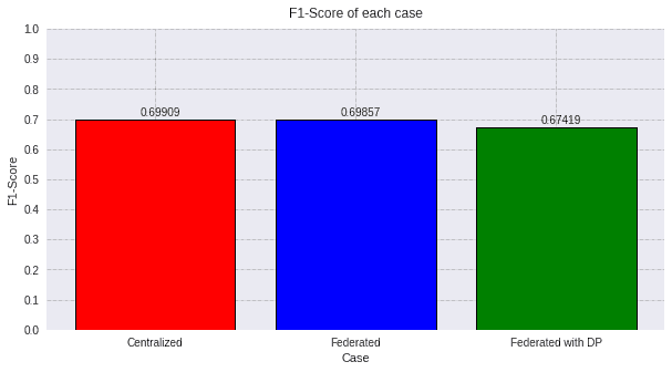
For a clear evaluation using the F1-score, we make predictions and we plot the results:

federated_model = federated_government._server._model
predictions_fed = federated_model.predict(test_data)

dp_model = federated_governmentDP._server._model
predictions_dp = dp_model.predict(test_data)


score_fed_f1 = f1_score(test_labels, predictions_fed, average='macro')
score_cent_f1 = f1_score(test_labels, predictions_cent, average='macro')
score_dp_f1 = f1_score(test_labels, predictions_dp, average='macro')


values=[round(score_cent_f1, 5), round(score_fed_f1, 5), round(score_dp_f1, 5)]
titles=['Centralized', 'Federated', 'Federated with DP']
colors=['red', 'blue', 'green']
plot_all_f1(values, titles, colors)

png

The most private model scores less than the others, as we are using low values of ε, which means high privacy. However, the performance loss is not really significant mantaining the model's utility.

5) Case with more features and classes

Below we present a more complex case, introducing more features and classes. When using more than two features, the figures are not plotted. Since the structure of the example is identical to the above, the comments are not repeated:

# Create database:
n_features = 11
n_classes = 5
n_samples = 10000
data, labels = make_classification(
    n_samples=n_samples, n_features=n_features, n_informative=4, 
    n_redundant=0, n_repeated=0, n_classes=n_classes, 
    n_clusters_per_class=2, weights=None, flip_y=0.1, class_sep=0.1, random_state=123)
database = WrapLabeledDatabase(data, labels)

train_data, train_labels, test_data, test_labels = database.load_data()
print("Shape of training and test data: " + str(train_data.shape) + str(test_data.shape))
print("Shape of training and test labels: " + str(train_labels.shape) + str(test_labels.shape))
print(train_data[0,:])

Shape of training and test data: (8000, 11)(2000, 11)
Shape of training and test labels: (8000,)(2000,)
[-8.46002695e-01 -1.16458262e-01  1.72024267e+00  2.49805434e-01
  9.94225074e-04 -2.46320085e+00  1.65177329e-01 -1.03454234e-01
  5.86144394e-01 -1.89988036e+00  2.37028165e-01]

5.1) Run the federated learning experiment

We run the federated learning training again with the new scenario.

iid_distribution = shfl.data_distribution.IidDataDistribution(database)
nodes_federation, test_data, test_labels = iid_distribution.get_nodes_federation(num_nodes=5, percent=100)

classes = np.unique(train_labels)
def model_builder():
    sk_model = LogisticRegression(warm_start=True, solver='lbfgs', multi_class='auto')
    model = LinearClassifierModel(n_features=n_features, classes=classes, model=sk_model)
    return model

aggregator = shfl.federated_aggregator.FedAvgAggregator()

federated_government = shfl.federated_government.FederatedGovernment(model_builder(), nodes_federation, aggregator)
federated_government.run_rounds(n_rounds=3, test_data=test_data, test_label=test_labels)

Evaluation in round 0:

Collaborative model test -> balanced_accuracy: 0.21695935748030432  cohen_kappa: 0.021965111749715605  

Evaluation in round 1:

Collaborative model test -> balanced_accuracy: 0.21695935748030432  cohen_kappa: 0.021965111749715605  

Evaluation in round 2:

Collaborative model test -> balanced_accuracy: 0.21695935748030432  cohen_kappa: 0.021965111749715605

5.2) Comparison with centralized training

We plot the decision boundaries and we calculate the results of the centralized case.

# Train model on centralized data:
model_centralized = LinearClassifierModel(n_features=n_features, classes=classes)
model_centralized.train(train_data, train_labels)
if n_features == 2:
    plot_2D_decision_boundary(model_centralized._server._model, train_data, train_labels, title = "Benchmark: Logistic regression using Centralized data")
print('Centralized test performance: ' + str(model_centralized.evaluate(test_data, test_labels)))

Centralized test performance: [('balanced_accuracy', 0.21777331793783974), ('cohen_kappa', 0.023074162189089975)]

5.3) Run the federated learning experiment with differential privacy

We calculate the sensitivity:

# Create sampling database:
n_samples = 10000
sampling_data, sampling_labels = make_classification(
    n_samples=n_samples, n_features=n_features, n_informative=4, 
    n_redundant=0, n_repeated=0, n_classes=n_classes, 
    n_clusters_per_class=2, weights=None, flip_y=0.1, class_sep=0.1, random_state=123)   
sample_data = np.hstack((sampling_data, sampling_labels.reshape(-1,1)))
distribution = UniformDistribution(sample_data)

# Sample sensitivity:
n_data_size = 300
max_sensitivity, mean_sensitivity = sampler.sample_sensitivity(
    LogisticRegressionSample(n_features=n_features, classes=classes), 
    L1SensitivityNorm(), distribution, n_data_size=n_data_size, gamma=0.05)
print("Max sensitivity from sampling: " + str(max_sensitivity))
print("Mean sensitivity from sampling: " + str(mean_sensitivity))

Max sensitivity from sampling: [0.10107813153343342, 0.741516015517064]
Mean sensitivity from sampling: [0.037309870445208906, 0.37895949355216857]

At this stage we are ready to add a layer of DP to our federated learning model and run again a federated training:

from shfl.differential_privacy import LaplaceMechanism

params_access_definition = LaplaceMechanism(sensitivity=max_sensitivity, epsilon=0.5)
nodes_federation.configure_model_params_access(params_access_definition)

federated_governmentDP = shfl.federated_government.FederatedGovernment(
    model_builder(), nodes_federation, aggregator)

federated_governmentDP.run_rounds(n_rounds=3, test_data=test_data, test_label=test_labels)

Evaluation in round 0:

Collaborative model test -> balanced_accuracy: 0.2030809084399065  cohen_kappa: 0.0011770724793949139  

Evaluation in round 1:

Collaborative model test -> balanced_accuracy: 0.20021071269265747  cohen_kappa: 0.0005059860457659049  

Evaluation in round 2:

Collaborative model test -> balanced_accuracy: 0.2114798955577521  cohen_kappa: 0.01574216585026811

5.4) F1-score comparison

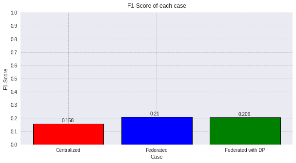
For a clear evaluation using the F1-score, we make predictions and we plot the results:

federated_model = federated_government._server._model
predictions_fed = federated_model.predict(test_data)

dp_model = federated_governmentDP._server._model
predictions_dp = dp_model.predict(test_data)


score_fed_f1 = f1_score(test_labels, predictions_fed, average='macro')
score_cent_f1 = f1_score(test_labels, predictions_cent, average='macro')
score_dp_f1 = f1_score(test_labels, predictions_dp, average='macro')


values=[round(score_cent_f1, 3), round(score_fed_f1, 3), round(score_dp_f1, 3)]
titles=['Centralized', 'Federated', 'Federated with DP']
colors=['red', 'blue', 'green']
plot_all_f1(values, titles, colors)

png

In this case, the problem is a lot more complicated than before, so a logistic regression is not enough to determine a proper prediction. In this case, we could generate predictions randomly and we would obtain a similar score.