Vertical Federated Learning with Sherpa.ai platform using PSI
Federated Learning is a Machine Learning paradigm aimed at learning models from decentralized data, such as data located on users’ smartphones, in hospitals, or banks, and ensuring data privacy. This is achieved by training the model locally in each node (e.g., on each smartphone, at each hospital, or at each bank), sharing the model-updated local parameters (not the data) and securely aggregating them to build a better global model.
Traditional Machine Learning requires all the data to be gathered in one single place. In practice, this is often forbidden by privacy regulations. For this reason, Federated Learning is introduced, the goal being to learn from a large amount of data, while preserving privacy.
The supported Federated Learning categories are: Horizontal, Vertical and Transfer. In this notebook, we will train by Vertical Federated Learning, where the nodes share overlapping samples (share the same sample ID space) but differ in data features. VFL employs this heterogeneity to train a more accurate model. The main idea to do this is to split a Neural Network among different parties and a server.
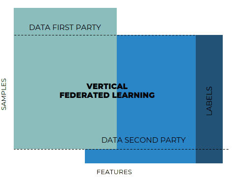
VFL requires the nodes to share overlapping samples, i.e. the two clients must have the same samples in the same oder (the first row of the first client must match with the first row of the second client, etcetera...). In practice, this assumption is not verified. To reduce to such assumption, we perform Private Set Intersection (PSI) or Privacy Preserving Entity Resolution (PPER).
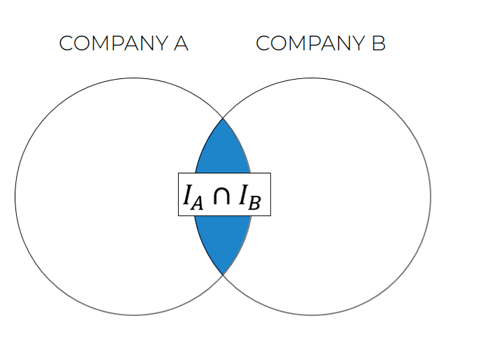
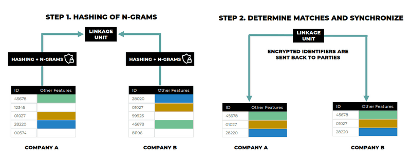
In this procedure, encrypted identifiers (e.g. email, card ID...) are shared between the parties to enable each company to link the customers they have in common before the training of the local models. As only encrypted identifiers are shared, both customers’ identifiers and the other private features (e.g. age, salary, postal code) of each company are kept safe. The identifier can be a composition of two or more variables with a certain transformation. This can lead to more security as the raw identifier is not shared.
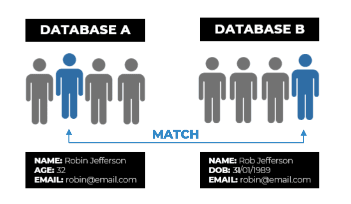
Nevertheless, Company A may be able to know which clients it has in common with Company B. The same applies the other way around. Technically speaking, PSI would make sample identifiers of the intersection visible to all parties, and therefore each party can know that the data entities shown in the intersection also appear in the other parties. Nonetheless, neither of the companies can obtain the data from the other company, information regarding the clients stays safe.
On the one hand, there are cases case where this membership information leakage is allowed between the companies. On the other hand, In some other cases, this membership information is sensitive and must be protected because of privacy standards and regulations.
In our case, we assume that the bank and the insurance have the agreement of knowing the sample ID of the intersection.
In this notebook we will simulate a fictional scenario where a Bank and an Insurance Company want to collaborate to train a model using Sherpa.ai's platform in a private way that will allow to predict the likelihood of a bank's client to subscribe to a long-term deposit without compromising any data.
The general description of the problem is:
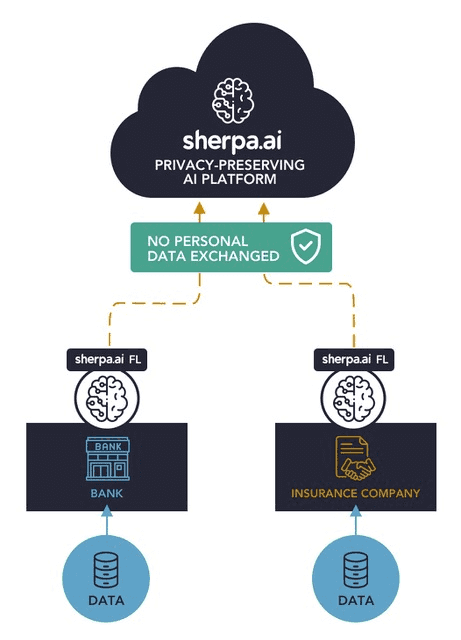
Using the the dataset Bank marketing campaigns dataset and in order to simulate a vertically partitioned training data, we will use some of the features as the data of one client (bank), and the rest for the other client (insurance).
Importance of the prediction of the output label:
A label (class label, output, prediction, target, or response) is the special attribute to be predicted based on all the input attributes.
A general description of the data:
Bank's data:
- 1 - age: Age of the lead (numeric)
- 2 - job: Type of job (categorical: "admin.","blue-collar","entrepreneur","housemaid","management","retired","self-employed","services","student","technician","unemployed","unknown")
- 3 - marital: Marital status (categorical: "divorced","married","single","unknown"; note: "divorced" means divorced or widowed)
- 4 - education (categorical: "basic.4y","basic.6y","basic.9y","high.school","illiterate","professional.course","university.degree","unknown")
- 5 - default: Does the lead have any default (unpaid) credit? (categorical: "no","yes","unknown")
- 6 - housing: Does the lead have any housing loan? (categorical: "no","yes","unknown")
- 7 - loan: Does the lead have any personal loan? (categorical: "no","yes","unknown")
- 8 - label - Has the client subscribed a term deposit? (binary: "yes","no")
Insurance's data:
- 9 - contact: Contact communication type (categorical: "cellular","telephone")
- 10 - month: Last contact month of year (categorical: "jan", "feb", "mar", …, "nov", "dec")
- 11 - dayofweek: Last contact day of the week (categorical: "mon","tue","wed","thu","fri")
- 12 - campaign: number of contacts performed during this campaign and for this client (numeric, includes last contact)
- 13 - pdays: Number of days that passed by after the client was last contacted from a previous campaign (numeric; 999 means client was not previously contacted)
- 14 - previous: Number of contacts performed before this campaign and for this client (numeric)
- 15 - poutcome: Outcome of the previous marketing campaign (categorical: "failure","nonexistent","success")
- 16 - emp.var.rate: employment variation rate - quarterly indicator (numeric)
- 17 - cons.price.idx: Consumer price index - monthly indicator (numeric)
- 18 - cons.conf.idx: Consumer confidence index - monthly indicator (numeric)
- 19 - euribor3m: Euribor 3 month rate - daily indicator (numeric)
- 20 - nr.employed: Number of employees - quarterly indicator (numeric)
VFL requires the nodes to share overlapping samples, i.e. the two clients must have the same samples in the same oder (the first row of the first client must match with the first row of the second clients, etcetera...). In practice, this assumption is not verified. To reduce to such assumption, we perform Private Set Intersection (PSI) or Privacy Preserving Entity Resolution (PPER).
Once that we have a general overview of our problem, the procedure is the following:
Index
As we can see, the preprocessing in this case is done after we do the PSI.
0) Libraries and data
import warnings
import matplotlib.pyplot as plt
import pandas as pd
import torch
import torch.nn as nn
from shfl.auxiliar_functions_for_notebooks import intersection_federated_government
from shfl.auxiliar_functions_for_notebooks.data_splitting import *
from shfl.auxiliar_functions_for_notebooks.functionsFL import *
from shfl.auxiliar_functions_for_notebooks.node_initialization import nodes_list, nodes_federation
from shfl.auxiliar_functions_for_notebooks.preprocessing import *
from shfl.data_base.data_base import split_train_test
from shfl.federated_aggregator import FedSumAggregator
from shfl.federated_government.vertical_federated_government import VerticalFederatedGovernment
from shfl.model.vertical_deep_learning_model_pt import VerticalNeuralNetClientModelPyTorch
from shfl.model.vertical_deep_learning_model_pt import VerticalNeuralNetServerModelPyTorch
from shfl.private.reproducibility import Reproducibility
from shfl.private.federated_operation import NodesFederation


plt.style.use('seaborn')
pd.set_option("display.max_rows", 30, "display.max_columns", None)
warnings.filterwarnings('ignore')
Reproducibility(567)
2022-04-25 11:45:20.821021: W tensorflow/stream_executor/platform/default/dso_loader.cc:64] Could not load dynamic library 'libcudart.so.11.0'; dlerror: libcudart.so.11.0: cannot open shared object file: No such file or directory
2022-04-25 11:45:20.821037: I tensorflow/stream_executor/cuda/cudart_stub.cc:29] Ignore above cudart dlerror if you do not have a GPU set up on your machine.
1 nodes_list= <shfl.private.federated_operation.HeterogeneousDataNode object at 0x7f0ca029a0d0>
1 nodes_list= <shfl.private.federated_operation.HeterogeneousDataNode object at 0x7f0bde92b850>
1 nodes_list= <shfl.private.federated_operation.VerticalServerDataNode object at 0x7f0c9d6491f0>
<shfl.private.reproducibility.Reproducibility at 0x7f0c9f39a160>We load the data of the bank and the insurance:
data_bank_total = pd.read_csv("./data_bank.csv", sep=",")
data_insurance_total = pd.read_csv("./data_insurance.csv", sep=",")data_bank_total.head()| age | job | marital | education | default | housing | loan | label | |
|---|---|---|---|---|---|---|---|---|
| 0 | 35 | entrepreneur | married | basic.9y | no | yes | no | no |
| 1 | 36 | blue-collar | divorced | basic.9y | unknown | no | no | no |
| 2 | 40 | entrepreneur | married | university.degree | no | no | no | no |
| 3 | 42 | services | married | high.school | no | no | no | no |
| 4 | 25 | student | single | high.school | no | yes | yes | yes |
The clients' data are the one that we have already described, so we show the first rows of the data:
data_insurance_total.head()| campaign | pdays | previous | emp.var.rate | cons.price.idx | cons.conf.idx | euribor3m | nr.employed | contact | month | day_of_week | poutcome | |
|---|---|---|---|---|---|---|---|---|---|---|---|---|
| 0 | 1 | 999 | 0 | -1.7 | 94.027 | -38.3 | 0.890 | 4991.6 | telephone | aug | wed | nonexistent |
| 1 | 2 | 999 | 0 | 1.4 | 94.465 | -41.8 | 4.961 | 5228.1 | telephone | jun | thu | nonexistent |
| 2 | 1 | 999 | 0 | 1.4 | 93.918 | -42.7 | 4.963 | 5228.1 | cellular | jul | wed | nonexistent |
| 3 | 3 | 999 | 0 | 1.1 | 93.994 | -36.4 | 4.855 | 5191.0 | telephone | may | fri | nonexistent |
| 4 | 2 | 6 | 3 | -1.7 | 94.055 | -39.8 | 0.761 | 4991.6 | cellular | jun | tue | success |
1) Prepare the data for a vertical federated learning scenario with PSI
As we want to show that the PSI works, we are going to take some random samples for each of the parties. This way, there will be samples that are exclusive for the bank, and other samples exclusives for the insurance. The objetive is to match those variable that are common between the clients.
To do the entity matching, we have to select a variable (or some variables) which uniquely correspond to the same instance. This matching is going to be done through a variable ID, that we will add to our datasets.
We select a portion of the data of the bank:
portion_data_bank = get_subsample(data_bank_total, int(data_bank_total.shape[0] * 0.98))portion_data_bank.to_csv("data_bank_subsampled.csv", index=True, index_label="ID")We select a portion of the data of the insurance:
portion_data_insurance = get_subsample(data_insurance_total, int(data_insurance_total.shape[0] * 0.96))portion_data_insurance.to_csv("data_ins_subsampled.csv", index=True, index_label="ID")data_bank = pd.read_csv("./data_bank_subsampled.csv", sep=",")
data_ins = pd.read_csv("./data_ins_subsampled.csv", sep=",")print('There are {} observations with {} features for the bank.'.format(data_bank.shape[0], data_bank.shape[1]))
print('There are {} observations with {} features for the insurance.'.format(data_ins.shape[0], data_ins.shape[1]))There are 40364 observations with 9 features for the bank.
There are 39540 observations with 13 features for the insurance.As we can observe, there are not the same number of instances for the bank node and the insurance node. With the PSI, we will work only with the intersection of those observations, this is, the instances that are both in the bank and in the insurance.
data_bank.head()| ID | age | job | marital | education | default | housing | loan | label | |
|---|---|---|---|---|---|---|---|---|---|
| 0 | 40535 | 61 | admin. | married | unknown | no | no | no | yes |
| 1 | 11363 | 34 | technician | divorced | professional.course | no | yes | no | no |
| 2 | 16506 | 41 | technician | divorced | university.degree | no | yes | no | no |
| 3 | 1743 | 27 | admin. | single | high.school | no | yes | no | no |
| 4 | 39982 | 33 | blue-collar | single | basic.6y | no | yes | no | yes |
data_ins.head()| ID | campaign | pdays | previous | emp.var.rate | cons.price.idx | cons.conf.idx | euribor3m | nr.employed | contact | month | day_of_week | poutcome | |
|---|---|---|---|---|---|---|---|---|---|---|---|---|---|
| 0 | 11359 | 1 | 999 | 0 | -1.8 | 93.075 | -47.1 | 1.405 | 5099.1 | cellular | apr | fri | nonexistent |
| 1 | 24851 | 7 | 999 | 0 | -1.8 | 92.893 | -46.2 | 1.244 | 5099.1 | cellular | may | mon | nonexistent |
| 2 | 34320 | 2 | 999 | 0 | 1.1 | 93.994 | -36.4 | 4.857 | 5191.0 | telephone | may | tue | nonexistent |
| 3 | 8259 | 2 | 999 | 1 | -1.8 | 92.893 | -46.2 | 1.281 | 5099.1 | cellular | may | wed | failure |
| 4 | 16287 | 1 | 999 | 0 | 1.4 | 93.444 | -36.1 | 4.965 | 5228.1 | cellular | aug | wed | nonexistent |
We can also notice that the instances are not aligned. PSI will be in charge of align the matches in a private preserving manner.
The server, that in this case corresponds to the bank, will have the labels
data_server = data_bank[["ID", "label"]]2) PSI
2.1) Execute PSI
In node_initialization, nodes in nodes_list are endowed with tools (functions, data structures) to perform hashing and PSI and Vertical Federated Learning (VFL).
Note that the first node (client node) and the last node (server node) are supposed to be mounted in the same physical node (the bank, who has the labels).
nodes_list[0].set_private_data(data_bank)nodes_list[1].set_private_data(data_ins)nodes_list[2].set_private_data(data_server)As we have presented, PSI is a technique aimed at determining the intersection of two private sets, without sharing the elements of such sets.
In our case, the goal is to determine the intersection of identifiers sets and (e.g. e-mail, ID-card number or name) of samples of datasets owned by different parties, without sharing identifiers values. Indeed, an identifier may be private.
Once the intersection is determined, intersecting identifiers are ordered, so aligning datasets belonging to different organizations.
p = 1048343
feast_list=["ID"]

intersection_federated_government.run_intersection(nodes_list, feast_list, p)
STEP 1. Hash identifiers onto Z_p.
STEP 2. First checks and parameters definition.
STEP 3. Send encrypted identifiers to the server.
STEP 4. Compute intersection hashed identifiers.And now we can synchronize the datasets:
n=2
for k in range(n + 1):
nodes_list[k].call('synchronize_dataset')Now we will obtain the intersection manually without caring about privacy. This will help us later to evaluate how accurate the PSI was performed in comparison with a non-private intersection:
intersected_centralized_data = data_bank.merge(data_ins, how = 'inner', on = 'ID')The SI without any kind of privacy, gives that the number of elements that are common in the bank and the insurance are:
#np means no privacy
inters_np = intersected_centralized_data["ID"].tolist()len(inters_np)38745This means that the porcentaje of data of each node that were not in common with the other party are:
round(100-(len(inters_np)*100 / data_bank.shape[0]),3)4.011round(100-(len(inters_np)*100 / data_ins.shape[0]),3)2.011This means that not all the data of each party will be used in the training. Just the data that is intersected.
To have a benchmark of the performance of federated learning in comparison with a non-private centralized case, we are going to join this already shuffled and intersected datasets. Obviously, this is done just for study and must be forbidden in a real world scenario.
labels_bank_for_comparison = nodes_list[0].query()["label"]labels_bank_for_comparison = label_encoder(labels_bank_for_comparison)data_bank_for_comparison = nodes_list[0].query().drop(["ID", "label"], axis=1)data_ins_for_comparison = nodes_list[1].query().drop(["ID"], axis=1)centralized_datasets = pd.concat([data_bank_for_comparison.reset_index(drop=True), data_ins_for_comparison], axis=1)As we mentioned, now we will compare the resulting intersections obtained by PSI with the real intersections. Some collisions may occur when hashing the identifiers resulting in some misaligned rows. In particular, there may be:
- false positives, due to collision of intersecting encrypted identifier, with non intersecting one.
- false negatives, due to collision of two intersecting encrypted identifiers.
inters_p_1 = nodes_list[0].query()['ID'].tolist()
print(len(inters_p_1))
print(len(list(set(inters_p_1).intersection(inters_np)))/len(inters_np))
38037
0.9809523809523809inters_p_2 = nodes_list[1].query()['ID'].tolist()
print(len(inters_p_2))
print(len(list(set(inters_p_2).intersection(inters_np)))/len(inters_np))38037
0.9813653374628984The elements that are the same in the bank and the insurance and coincides with the one of the non-private set intersection is:
len([i for i, j in zip(inters_p_1, inters_p_2) if i == j])37655This means that the real matches are 38745 but with PSI we match 38037. Almost 700 instances have been lost because of these collisions.
From those 38037 matches, 37655 are real matches, so almost 400 matches are false positives.
The percentaje shows how many elements of each party are real intersections, this is, coincides with the non private set intersection .
In the remainder, we are going to test our privacy-preserving Federated Learning technology. In the spirit of privacy preservation, we set up a more strict access policy.
def privacy_preserving_query(dataset):
    """Returns only the number of columns of dataset. """
    return dataset.data.shape[1]

n = 2
for i in range(n + 1):
    nodes_list[i].configure_data_access(privacy_preserving_query)
2.3) Data preprocessing
Now that the data are correctly aligned we should preprocess it. The preprocessing will consist in:
- Drop the ID variable since it is only used to do the matching
- If necessary, split the data into inputs and labels.
- Convert non-numeric categorical columns to one hot encoding format.
- Normalize the numeric columns
- Transform pandas.DataFrame into numpy.ndarray.
That will be done with transform_data, a function inside the nodes:
nodes_list[0].call('transform_data', label_name='label', id_name= "ID")nodes_list[1].call('transform_data', label_name='label', id_name= "ID")nodes_list[2].call('transform_data', label_name='label', id_name= "ID")And as the final step, we can internally split the data in train and test in each node. In PSI, the cardinality of the intersection is known for the clients. As they have synchronized their datasets, the orchestator can send the order to take a portion for training and a portion of testing for each client. In this case, the portion will be the 80% first columns:
nodes_list[0].call('split_train_test', train_proportion=0.8)nodes_list[1].call('split_train_test', train_proportion=0.8)nodes_list[2].call('split_train_test', train_proportion=0.8, is_label=True)3) Run the experiment
Now we are going to execute the federated, local and centralized experiments in order to compare the results and illustrate how the model's metrics behave in these scenarios. As in the notebook explaining the basic concepts of vFL, we are going to emulate the process of creating the whole structure and we will train the models.
3.1) Federated
client_out_dim = 2

model0 = nn.Sequential(
    nn.Linear(nodes_list[0].query(), client_out_dim, bias=True),
)

model1 = nn.Sequential(
    nn.Linear(nodes_list[1].query(), client_out_dim, bias=True),
)

optimizer0 = torch.optim.SGD(params=model0.parameters(), lr=0.001)
optimizer1 = torch.optim.SGD(params=model1.parameters(), lr=0.001)

batch_size = 32
model_nodes = [VerticalNeuralNetClientModelPyTorch(model=model0, loss=None, optimizer=optimizer0, batch_size=batch_size),
               VerticalNeuralNetClientModelPyTorch(model=model1, loss=None, optimizer=optimizer1, batch_size=batch_size)]
# Define the model of the server node
model_server = torch.nn.Sequential(
torch.nn.Linear(client_out_dim, 1, bias=True),
torch.nn.Sigmoid())
loss_server = torch.nn.BCELoss(reduction="mean")
optimizer_server = torch.optim.SGD(params=model_server.parameters(), lr=0.001)
model = VerticalNeuralNetServerModelPyTorch(model_server, loss_server, optimizer_server,
metrics={"accuracy":accuracy})
# Set the model and the aggregator in the server node
nodes_list[2].set_model(model)
nodes_list[2].set_aggregator(FedSumAggregator())
# Configure data access to nodes and server
nodes_federation.configure_model_access(meta_params_query)
nodes_list[2].configure_model_access(meta_params_query)
nodes_list[2].configure_data_access(train_set_evaluation)# Convert to float
nodes_federation.apply_data_transformation(cast_to_float);# Create federated government
federated_government = VerticalFederatedGovernment(model_nodes,
nodes_federation,
server_node=nodes_list[2])
# Run training and testing
federated_government.run_rounds(n_rounds=10001,
eval_freq=1000)Evaluation in round 0 :
Loss: 1.0554678440093994 Accuracy: 0.13040620481135795
Evaluation in round 1000 :
Loss: 0.7056271433830261 Accuracy: 0.5016432233469174
Evaluation in round 2000 :
Loss: 0.5098281502723694 Accuracy: 0.843302221637965
Evaluation in round 3000 :
Loss: 0.4000872075557709 Accuracy: 0.8845799921125279
Evaluation in round 4000 :
Loss: 0.3449161648750305 Accuracy: 0.890758511896937
Evaluation in round 5000 :
Loss: 0.31737613677978516 Accuracy: 0.8935191271197581
Evaluation in round 6000 :
Loss: 0.3032967150211334 Accuracy: 0.896542658078086
Evaluation in round 7000 :
Loss: 0.2952573895454407 Accuracy: 0.8990403575654002
Evaluation in round 8000 :
Loss: 0.290302038192749 Accuracy: 0.8993032733009071
Evaluation in round 9000 :
Loss: 0.28683537244796753 Accuracy: 0.8996976469041672
Evaluation in round 10000 :
Loss: 0.2843988835811615 Accuracy: 0.9006178519784409y_prediction_fed = nodes_list[2].call('plot_roc')
3.2) Local (Data from the bank only)
The local case refers to the situation where we only have the data belonging to one of the clients, which in this case is the bank. This will be useful to understand how the insurance data improves the metric of the model obtained by using only the data of the bank. We have to comment that the data should always remain inside the node. As this is an experimental notebook to illustrate the federated experiment and doing a comparison, we will use the test data of the local party (the bank), but keep in mind that this operation is done locally by one party.
local_data = preprocessing_data(data_bank_for_comparison)train_data_bank, train_labels, test_data_bank, test_labels = split_train_test(local_data,
labels_bank_for_comparison)y_prediction_loc = sklearn_logistic_predictions(train_data_bank, train_labels, test_data_bank)y_prediction_loctest_labelsarray([0, 0, 1, ..., 0, 0, 0])plot_roc(y_prediction_loc, test_labels)
3.3) Centralized (Data joined without any privacy)
The centralized data represents a node that has the whole dataset, joined without any kind of privacy. In principle, this will imply a better accuracy but, for sure, this can not happen in a real world scenario, where the data are dispersed over different organizations under the protection of privacy restrictions. We will load the centralized data, joining the two datasets that have been matched with a non private SI.
centralized_data = preprocessing_data(centralized_datasets)train_centralized_data, test_centralized_data = split_train_test(centralized_data)
y_prediction_cent = sklearn_logistic_predictions(train_centralized_data, train_labels, test_centralized_data)plot_roc(y_prediction_cent, test_labels)
3.4) Comparison
3.4.1) ROC curve
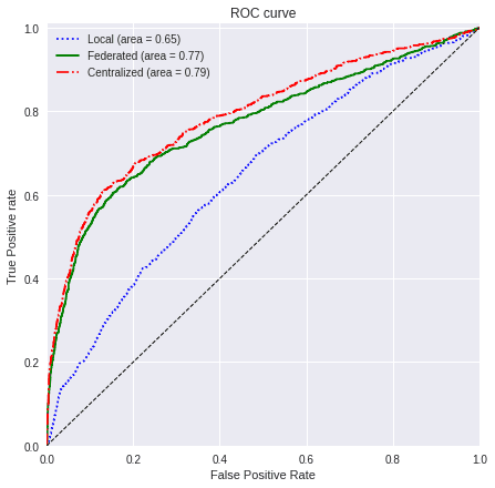
With the next function, we will plot a comparison between the metric of the three cases that we have presented:
values=[y_prediction_loc, y_prediction_fed, y_prediction_cent]
titles=['Local', 'Federated', 'Centralized']
colors=['blue', 'green', 'red']
linestyle=[':','-','-.']

plot_all_roc_curves(test_labels, values, titles, colors, linestyle)
3.4.2) F1-Score
n_classes=2

values_f1_fed = (y_prediction_fed > 0.5).astype(int)

values_f1_loc = (y_prediction_loc > 0.5).astype(int)

values_f1_cent = (y_prediction_cent > 0.5).astype(int)


score_fed_f1 = f1_score(test_labels, values_f1_fed, average='macro')

score_loc_f1 = f1_score(test_labels, values_f1_loc, average='macro')

score_cent_f1 = f1_score(test_labels, values_f1_cent, average='macro')


values=[round(score_loc_f1, 3), round(score_fed_f1, 3), round(score_cent_f1, 3)]
titles=['Local', 'Federated', 'Centralized']
colors=['blue', 'green', 'red']
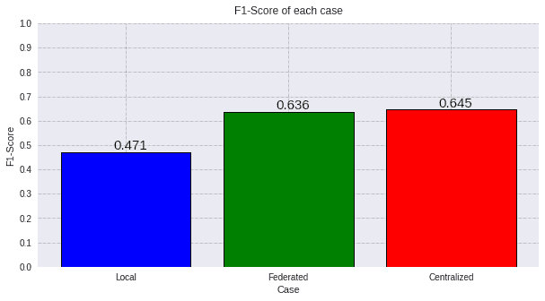
plot_all_metric(values, "F1-Score", titles, colors)
These figure show three different results:
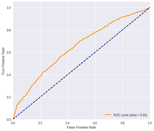
- In , we have the result of using just the local data of the bank. This correspond to the local case, where we have the features of the bank but not the insurance.
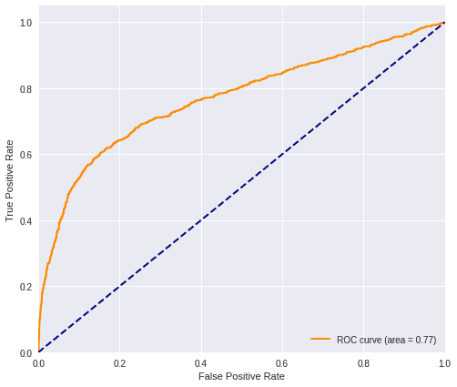
- In , we have the result of the federate experiment, where we have used the features of both clients in a privacy preserving manner using Private Set Intersection.
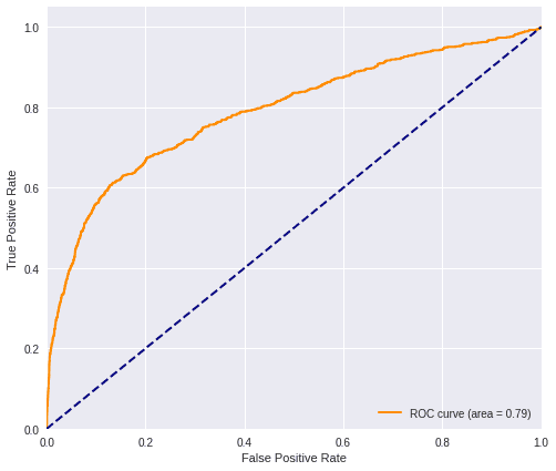
- In , we have the result of using the centralized data aggregation of both clients without any kind of privacy.
The figures show the benefit of using the data of both clients in a privacy preserving manner in comparison with just one client. Even though the best scenario in term of the metric is where we use the data in a centralized way, the improvement with respect to the federated case is not really significant, since it is really similar (only 0.02 higher regarding the ROC AUC and 0.005 regarding the F1 score)
In summary, by using linear models in the nodes, the results of the ROC AUC for the three different cases are:
Local (0.65) << Federated (0.77) < Centralized (0.79)
We improve by 0.13 the prediction of the bank by using the data of the insurance in a federated way while preserving the privacy. By using all the data BUT without preserving the privacy, we would only improve a 0.02 with respect to the federated model.
And the results of the F1 score are:
Local (0.471) << Federated (0.636) < Centralized (0.645)
We improve by 0.165 the prediction of the bank by using the data of the insurance in the federated way. By using all the data BUT without preserving the privacy, we would only improve a 0.005 with respect to the federated model.
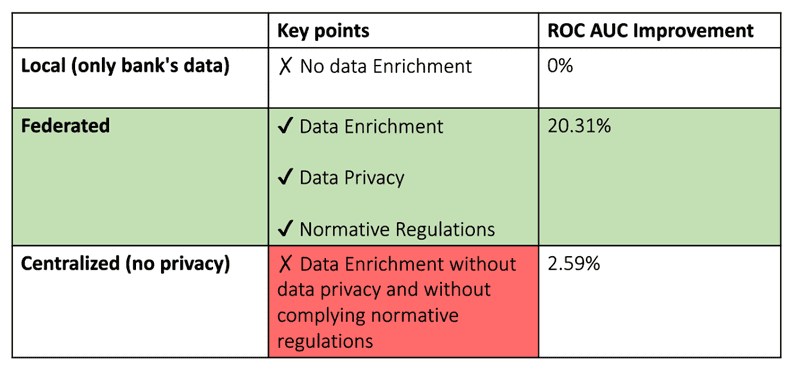
The model trained with the bank's data solely has no data enrichment, whereas the federated one enjoys data enrichment, data privacy and complies with all the normative regulations, apart from having a greater accuracy improvement.
As a conclusion of this notebook, we can notice the benefits of using the Sherpa.ai’s Privacy-Preserving platform in a Vertical Federated scenario where the data of different parties are not aligned. The prediction is almost as much accurate as traditional machine learning methods, but with the significant benefit of ensuring the privacy of data and regulatory compliance.
Furthermore, PSI has been proven to work properly, since the most of the data has been correctly aligned.