Federated models: non-linear kernel SVM classification
In the present notebook, the idea for a Federated non-linear support vector machine (SVM) classification is presented. The model is encapsulated in the Sherpa.ai Federated Learning Framework on for a synthetic database. Moreover, differential privacy is applied and its impact on the global model is assessed.
Index
1) The data
We start by creating a synthetic database:
import shfl
from shfl.data_base.data_base import WrapLabeledDatabase
from sklearn.datasets import make_classification
import numpy as np
from shfl.model.linear_classifier_model import LinearClassifierModel
from shfl.model.svm_classifier_model import SVMClassifierModel
from shfl.auxiliar_functions_for_notebooks.functionsFL import *
import numpy as np
from sklearn.svm import NuSVC
from sklearn.svm import SVC
from sklearn import metrics

# Create database:
n_features = 2
n_classes = 3
data, labels = make_classification(
    n_samples=10000, n_features=n_features, n_informative=2,
    n_redundant=0, n_repeated=0, n_classes=n_classes,
    n_clusters_per_class=1, weights=None, flip_y=0.1, class_sep=0.5)
database = WrapLabeledDatabase(data, labels)

train_data, train_labels, test_data, test_labels = database.load_data()

C = 1
kwargs = {'C':C, 'kernel':"linear"}
model_use = SVC(**kwargs)
2022-03-24 17:58:17.400626: W tensorflow/stream_executor/platform/default/dso_loader.cc:64] Could not load dynamic library 'libcudart.so.11.0'; dlerror: libcudart.so.11.0: cannot open shared object file: No such file or directory
2022-03-24 17:58:17.400664: I tensorflow/stream_executor/cuda/cudart_stub.cc:29] Ignore above cudart dlerror if you do not have a GPU set up on your machine.print("Shape of train and test data: " + str(train_data.shape) + str(test_data.shape))
print("Shape of train and test labels: " + str(train_labels.shape) + str(test_labels.shape))Shape of train and test data: (8000, 2)(2000, 2)
Shape of train and test labels: (8000,)(2000,)2) The model
Next, we define the new class for SVM using sklearn's Support Vector Machine classifiers.
By the implementation below, you can use either SVC or NuSVC:
# from shfl.model.utils import check_initialization_classification
# from shfl.model.utils import check_data_features
As reference, we train a centralized model (i.e. non-federated). And in the case of two features, we can visualize the solution on a plane:
# Train global model using framework's class:
classes = [i for i in range(0,n_classes)]
model_centralized = SVMClassifierModel(n_features=n_features, classes=classes, model=model_use)
model_centralized.train(data=train_data, labels=train_labels)
if n_features == 2:
    plot_2D_decision_boundary(model_centralized, test_data, labels=test_labels, title = "Benchmark: Classification using Centralized data")
print("Test performance using centralized data: " + str(model_centralized.evaluate(test_data, test_labels)))


predictions_cent = model_centralized.predict(test_data)

Test performance using centralized data: [('balanced_accuracy', 0.6690983355230552), ('cohen_kappa', 0.5051932152815586)]2.1) How to _aggregate a model's parameters from each federated node
sklearn provides three options for classification: LinearSVC, SVC and NuSVC.
The linear version LinearSVC is easily incorporated in the platform, since the aggregation of the model is straightforward (see notebook for Federated Logistic Regression, in which LinearSVC can be used instead of the logistic regression).
On the other hand, for SVC and NuSVC, the output model's parameters are more complex, since they depend on the number of support vectors for each class.
Thus, in principle, each client would deliver parameters with different dimensions, which are not straightforward to _aggregate.
Here, we use the clients' support vectors to train a global model directly on the server, obtaining the aggregated model:
import numpy as np
import inspect


def svm_aggregator(clients_params):
    """Uses the server's (caller object) model to _aggregate the client's parameters."""
    caller_object = inspect.currentframe().f_back.f_locals['self']
    clients_params_array = np.vstack(clients_params)
    caller_object._model.train(clients_params_array[:, 0:-1], clients_params_array[:, -1].astype(int))

    return caller_object._model.get_model_params()
3) Run the federated learning experiment
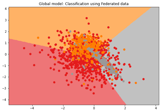
Once defined the aggregator, we can run the federated model. Note that the decision boundary can vary even by running the training on the same data (this is due to the internal shuffle of the data of the SVM solver). Thus, in order to compare the centralized and the federated models, it is more relevant to compare the scores on the test data:
iid_distribution = shfl.data_distribution.IidDataDistribution(database)
nodes_federation, test_data, test_labels = iid_distribution.get_nodes_federation(num_nodes=20, percent=100)

classes = [i for i in range(0,n_classes)]
def model_builder():
    model = SVMClassifierModel(n_features=n_features, classes=classes, model=model_use)
    return model

# aggregator = GlobalModelAggregator(SVMClassifierModel(n_features=n_features, classes=classes))
aggregator = svm_aggregator

federated_government = shfl.federated_government.FederatedGovernment(model_builder(), nodes_federation, aggregator)federated_government.run_rounds(n_rounds=3, test_data=test_data, test_label=test_labels)
if n_features == 2:
plot_2D_decision_boundary(federated_government._server._model,
test_data, test_labels,
title = "Global model: Classification using Federated data")Evaluation in round 0:
Collaborative model test -> balanced_accuracy: 0.6711961943239064 cohen_kappa: 0.5082788104256921
Evaluation in round 1:
Collaborative model test -> balanced_accuracy: 0.6701208304105807 cohen_kappa: 0.5067053481863151
Evaluation in round 2:
Collaborative model test -> balanced_accuracy: 0.6696095829668179 cohen_kappa: 0.5059459443200327

4) Add differential privacy
In instance-based machine learning methods such as SVM or KNN, part of the data (or the entire data, in the worst case) constitute the resulting model. These methods are thus particularly exposed to reconstruction attacks (e.g. see Yang et al. 2019). In order to protect private information, we can apply Differential Privacy on the resulting model output from the clients and observe its influence on the federated global model.
4.1) Sensitivity by sampling
We first estimate model's sensitivity by sampling. Recall that the matrices of support vectors are the actual models' parameters, and that they can have differing number of rows. We then need to define a distance between such matrices: we can choose the max of the Euclidean distance of their rows (see matrix distance).
Note that the sk-learn SVM solver is non-deterministic. In fact, due to the internal data shuffle, the SVM solver may deliver slightly different support vectors when training on the same set. Moreover, even when setting the random seed (see random_state input parameter), and simply switching one row in the training dataset, may result in slightly different output.
from shfl.differential_privacy import SensitivitySampler
from shfl.differential_privacy import L1SensitivityNorm
from shfl.differential_privacy import SensitivityNorm
from scipy.spatial import distance_matrix

class UniformDistribution(shfl.differential_privacy.ProbabilityDistribution):
    """
    Implement Uniform sampling over the data
    """
    def __init__(self, sample_data):
        self._sample_data = sample_data

    def sample(self, sample_size):
        row_indices = np.random.choice(a=self._sample_data.shape[0], size=sample_size, replace=False)

        return self._sample_data[row_indices, :]


class SVMClassifierSample(SVMClassifierModel):

    def __call__(self, data_array):
        data = data_array[:, 0:-1]
        labels = data_array[:, -1].astype(int)
        params = np.array([], dtype=np.int64).reshape(0, (self._n_features + 1))
        self.set_model_params(params)
        train_model = self.train(data, labels)
        model_params = self.get_model_params()
        model_params = model_params[:,0:-1] # Exclude the classes indices

        return model_params.copy()


class MatrixSetXoRNorm(SensitivityNorm):
    """
    Distance matrix using only rows not in common.
    """
    def compute(self, x_1, x_2):
        nrows, ncols = x_1.shape
        dtype = {'names':['f{}'.format(i) for i in range(ncols)],
                   'formats':ncols * [x_1.dtype]}
        x = np.setxor1d(x_1.view(dtype), x_2.view(dtype))
        x = x.view(x_1.dtype).reshape(-1, ncols)
        if x.shape[0] is not 0:
            x = distance_matrix(x,x)
            x = x.max()
        else:
            x = 0

        return x
<>:43: SyntaxWarning: "is not" with a literal. Did you mean "!="?
<>:43: SyntaxWarning: "is not" with a literal. Did you mean "!="?
/tmp/ipykernel_935822/2118452112.py:43: SyntaxWarning: "is not" with a literal. Did you mean "!="?
if x.shape[0] is not 0:As a matter of fact, in the sensitivity sampling, we consider databases that differ at most in one entry, or contain exactly the same data, yet some of the support vectors turn out to be different. This said, the sensitivity sampling procedure for this case is expected to deliver results with high variance.
The resulting sensitivity is particularly high, and the application of DP dramatically deteriorates the performance of the global model:
# Create sampling database:
n_instances = 400
sampling_data, sampling_labels = make_classification(
    n_samples=n_instances, n_features=n_features, n_informative=2,
    n_redundant=0, n_repeated=0, n_classes=n_classes,
    n_clusters_per_class=1, weights=None, flip_y=0.1, class_sep=0.1)
sample_data = np.hstack((sampling_data, sampling_labels.reshape(-1,1)))

# Sampling sensitivity:
distribution = UniformDistribution(sample_data)
sampler = SensitivitySampler()

n_data_size = 200 # must be <= n_instances
kwargs['random_state'] = 123
max_sensitivity, mean_sensitivity = sampler.sample_sensitivity(
    SVMClassifierSample(n_features=n_features, classes=classes, model=model_use),
    MatrixSetXoRNorm(), distribution, n_data_size=n_data_size, m_sample_size=100)

print("Max sensitivity from sampling: " + str(max_sensitivity))
print("Mean sensitivity from sampling: " + str(mean_sensitivity))
Max sensitivity from sampling: 4.884894520827751
Mean sensitivity from sampling: 1.36917179810165114.2) Run the federated learning experiment with differential privacy
At this stage we are ready to add a layer of DP to our federated learning model. The Gaussian mechanism is employed.
from shfl.differential_privacy import GaussianMechanism

sensitivity_array = np.full((n_features+1,), max_sensitivity)
sensitivity_array[-1] = 0  # We don't apply noise on the classes
params_access_definition = GaussianMechanism(sensitivity=sensitivity_array, epsilon_delta=(0.9, 0.9))
nodes_federation.configure_model_params_access(params_access_definition)

federated_governmentDP = shfl.federated_government.FederatedGovernment(
    model_builder(), nodes_federation, aggregator)

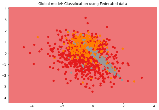
federated_governmentDP.run_rounds(n_rounds=1, test_data=test_data, test_label=test_labels)
if n_features == 2:
    plot_2D_decision_boundary(federated_governmentDP._server._model,
                              test_data, test_labels,
                              title = "Global model: Classification using Federated data")
Evaluation in round 0:
Collaborative model test -> balanced_accuracy: 0.3333333333333333 cohen_kappa: 0.0

4.3) Sensitivity associated to the data
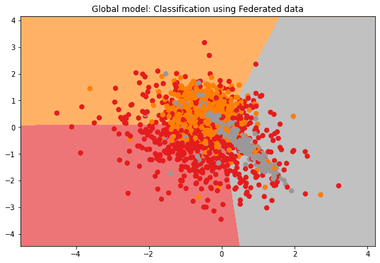
Since the SVM's parameters are constituted by the data itself, we might assume that the model's sensitivity is actually the sensitivity to apply on the data itself if one would try to access it. We then take the component-wise variance of the data as the sensitivity. The resulting -private global model's performance is then comparable to the non-private version:
from shfl.differential_privacy import GaussianMechanism

sensitivity_array = np.var(sample_data, axis=0)
sensitivity_array[-1] = 0  # We don't apply noise on the classes
print("Component-wise sensitivity: " + str(sensitivity_array))

params_access_definition = GaussianMechanism(sensitivity=sensitivity_array, epsilon_delta=(0.9, 0.9))
nodes_federation.configure_model_params_access(params_access_definition)

federated_governmentDP = shfl.federated_government.FederatedGovernment(
    model_builder(), nodes_federation, aggregator)

federated_governmentDP.run_rounds(n_rounds=1, test_data=test_data, test_label=test_labels)
if n_features == 2:
    plot_2D_decision_boundary(federated_governmentDP._server._model, test_data, test_labels, title = "Global model: Classification using Federated data")
Component-wise sensitivity: [0.61813351 1.09970295 0. ]
Evaluation in round 0:
Collaborative model test -> balanced_accuracy: 0.6315070166242993 cohen_kappa: 0.4480216645864218

4.4) F1-score comparison
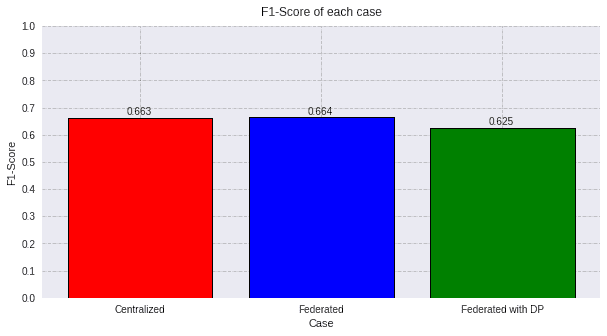
For a clear evaluation using the F1-score, we make predictions and we plot the results:
federated_model = federated_government._server._model
predictions_fed = federated_model.predict(test_data)

dp_model = federated_governmentDP._server._model
predictions_dp = dp_model.predict(test_data)

score_fed_f1 = f1_score(test_labels, predictions_fed, average='macro')
score_cent_f1 = f1_score(test_labels, predictions_cent, average='macro')
score_dp_f1 = f1_score(test_labels, predictions_dp, average='macro')


values=[round(score_cent_f1, 3), round(score_fed_f1, 3), round(score_dp_f1, 3)]
titles=['Centralized', 'Federated', 'Federated with DP']
colors=['red', 'blue', 'green']
plot_all_f1(values, titles, colors)

5) Remarks
Remark 1: Federated learning round. In this approach, the model's parameters are the actual support vectors. Thus, at each learning round, the support vectors are sent by the clients to the central server, where an additional SVM is run to _aggregate the global model. At that stage, the (global) support vectors are sent back to the clients and are used together with clients' data to train the local model. However, the global support vectors are not considered as local data, and thus are not stored as client's data on the node.
Remark 2: Application of DP. The model's sensitivity is highly responsive on the training data, and the resulting model's performance can be easily degenerated by application of DP. Sensitivity is computed both by sampling and data variance, and the former yields lower sensitivity.
Nevertheless, neither of the two approaches fit in the definition of sensitivity based on either L1 and L2 norms, and a more general notion of distance should be introduced for a formal guarantee of DP (see 3.3 in Dwork et al. 2016).
Remark 3: Reduction of training data. Since the SVM is particularly sensitive to duplicates in the training data, these are removed when fitting the model. However, when applying DP, there aren't essentially any identical instances and more sophisticated reduction techniques for training data should be used (e.g. a clustering technique as in Yu et al. 2003) since otherwise the set of training vectors would keep growing at each federated round and introducing excessive noise in the model. When DP is applied as in this approach, it is thus advisable to run only a few federated rounds.
Remark 4: Tuning for soft margin and kernel parameters. In the presented case default values are used, however a tuning is in general needed for SVM models.