⚠

Please note that these tutorials refer to a deprecated version of the platform. The current version of the platform, which is not publicly available, has a more advanced architecture and provides a wider range of functionalities. These tutorials are only for illustrative purposes and showcase a limited number of the platform’s capabilities.

Differential privacy: the exponential mechanism

In this notebook, we introduce the exponential mechanism (see The Algorithmic Foundations of Differential Privacy, Section 3.4). We consider three different examples that show how general the mechanism is.

Index

1) Exponential mechanism

Let $\mathcal{X}$ be the set of possible rows in a database so that we can represent a particular database using a histogram $x\in\mathbb{N}^{|\mathcal{X}|}$ . Given an arbitrary response space $\mathcal{R}$ and a utility function

u: \mathbb{N}^{|\mathcal{X}|}\times \mathcal{R} \rightarrow \mathbb{R}\,,

we define the exponential mechanism as the collection of conditional probabilities given by

P(r|x; u, \alpha) = \frac{e^{\alpha u(x,r) }}{\sum_{r'\in\mathcal{R}} e^{\alpha u(x,r')}}\,.

In the case of uncountable $\mathcal{R}$ , the sum in the denominator should be replaced with an integral and the expression above gives a probability density.

The exponential mechanism is an $\epsilon$ -differentially private randomization algorithm with $\epsilon = 2\alpha\Delta u$ and

\Delta u = \underset{r\in\mathcal{R}}{\rm max}\underset{||x-y||_1 \le 1}{\rm max} |u(x,r) - u(y,r)|\,.

The utility function, $u$ , can be thought of as a generalization of a numeric query. In fact, this mechanism can be reduced to simpler mechanisms for particular types of functions $u$ . In order to illustrate this, we will demonstrate how this works in two well-known examples.

2) Randomized response

Consider the case in which $\mathcal{R} = \{0, 1\}$ and $\mathcal{X} = \{\text{truly innocent}, \text{truly guilty}\}$ with a utility function such that

u(0, 0) = 0\qquad u(1, 0) = 0

u(0, 1) = \beta \qquad u(1, 1) = \gamma

where $\beta, \gamma$ are real constants. In this case, the exponential mechanism reduces to the simplest randomized response algorithm.

3) Laplace Mechanism

Consider the case in which $\mathcal{R} = \mathbb{R}$ and the utility function is given by $u(x, r) = -|f(x) - r|$ with

f: \mathbb{N}^{|\mathcal{X}|} \rightarrow \mathbb{R}\,.

This is, by definition, the Laplace mechanism with $b = \alpha^{-1}$ .

4) Example: the exponential mechanism to protect clients' bids

The input dataset $x$ is a set of bids for the purchase of an abundant supply of a product. The problem is to identify the best price $r \in \mathcal{R} = [r_{min}, r_{max}]$ so as to maximize the revenue, without revealing the bids. In this case the revenue is our utility function $u$ , defined as

u(x, r) = r |S_r|

with

S_r = \{i: x_i\ge r\}\,

the set of people that are willing to buy at a price $r$ .

In general, it is not possible to compute $\Delta u$ analytically and you must resort to statistical estimations of "typical" values of $\Delta u$ (see Rubinstein 2017). This is also the case when $\Delta u$ is not bounded. In our particular case, we can compute the sensitivity with respect to the utility, which is given by

\Delta u = r_{max}.

The complication in this case arises from the fact that the output price may not be directly perturbed. In Example 3.5 of The Algorithmic Foundations of Differential Privacy, they suppose there are four bidders: A, F, I, K, where A, F, I each bid 1.00 and K bids 3.01, so $x = \{1, 1, 1, 3.01\}$ . If we fix the price to 3.01, the revenue is $u=3.01$ , at $3.00$ we have $u=3.00$ , at $1.00$ we have $u=4.00$ . However, if we fix the price at $3.02$ , the revenue is zero! The revenue function for this specific demand defined by $x$ is shown below.

import matplotlib.pyplot as plt
import numpy as np
from scipy.stats import norm

def u(x, r):
    '''
    Utility function
    
    Arguments:
        x: list. True bids.
        r_range: array of possible values for the price.
    '''
    output = np.zeros(len(r))
    for i in range(len(r)): 
        output[i] = r[i] * sum(np.greater_equal(x, r[i]))
    return output

Using an imaginary dataset composed by the bids of the buyers and the intervals of possible prices, we calculate the resulting utility function:

x = [1.00, 1.00, 1.00, 3.01] # Input dataset: the true bids
r = np.arange(0, 3.5, 0.001) # Set the interval of possible outputs r


utility = u(x, r)

Now that the values are calculated, we only need to plot the utility (revenue) for each possible output r (price):

plt.style.use('fivethirtyeight')
fig, ax = plt.subplots(figsize=(9, 6))
x_intervals = np.sort(np.unique(np.append(x, [r.min(), r.max()])))
for i_interval in range(len(x_intervals) - 1):
    indices_interval = [all(union) for union in zip(
        r > x_intervals[i_interval], r <= x_intervals[i_interval + 1])]
    ax.plot(r[indices_interval], utility[indices_interval], color = "blue")

ax.set_xlim([r.min(), r.max()])
ax.set_xlabel('$r$')
ax.set_ylabel('Utility')
label="Utility (i.e. revenue) for all possible prices $r$"
ax.text(r.max()/2, -1, label, ha='center')

plt.show()

png

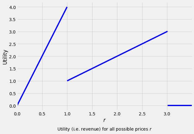
As explained above, the exponential mechanism is defined with respect to the utility function $u : \mathbb{N}^{|\mathcal{X}|} \times \mathcal{R} \rightarrow \mathbb{R}$ , which maps database/output pairs to utility scores. For a fixed database $x$ , the exponential mechanism outputs each possible $r \in \mathcal{R}$ with probability proportional to $\exp\left(\frac{\epsilon u\left(x, r\right)}{2\Delta u}\right)$ .

Here we got the definition of the Probability Density Function (PDF):

def PDF(x, r, epsilon):
    """
    PDF associated to the database x
    """
    r_min = r.min()
    r_max = r.max()    
    x_intervals = np.sort(np.unique(np.append(x, [r_min, r_max])))
    area = 0
    for i in range(len(x_intervals) - 1):
        S = epsilon/(2*r_max) * sum(np.greater(x, x_intervals[i]))
        if S > 0:
            area_int = 1/S * (np.exp(S * x_intervals[i + 1]) - np.exp(S * x_intervals[i]))
        elif S == 0:
            area_int = x_intervals[i + 1] - x_intervals[i]
        area = area + area_int
    
    u_prob_norm = np.exp(epsilon * u(x, r) / (2 * r_max)) / area
    return u_prob_norm

Now we need to establish the epsilon ranges to see how does distinct privacy budgets behave with the value ranges.

epsilon_range = [0.01, 1, 5]

The resulting probability distribution is shown in the plot below.

fig, ax = plt.subplots(figsize=(9,6))
color_list = ["b", "g", "r", "c", "m"]

x_intervals = np.sort(np.unique(np.append(x, [r.min(), r.max()])))
for i_epsilon in range(len(epsilon_range)):
    u_prob_norm = PDF(x, r, epsilon_range[i_epsilon])
    for i_interval in range(len(x_intervals) - 1):
        indices_interval = [all(union) for union in zip(
            r > x_intervals[i_interval], r <= x_intervals[i_interval + 1])]
        ax.plot(r[indices_interval], 
                u_prob_norm[indices_interval], 
                color = color_list[i_epsilon], 
                label = '$\epsilon = $' + str(epsilon_range[i_epsilon]))

handles, labels = ax.get_legend_handles_labels()  
handles = handles[0:len(handles):(len(x)-1)]
labels = labels[0:len(labels):(len(x)-1)]
ax.set_xlim([r.min(), r.max()])
ax.set_ylim([-0.1, max(u_prob_norm) + 0.1])
ax.set_xlabel('$r$')
ax.set_ylabel('Probability density')
ax.legend(handles, labels)
label="Probability density function for different levels of privacy $\epsilon$. For higher levels of privacy (i.e. lower $\epsilon$), \n\
the probability resembles the uniform distribution, while for lower levels of privacy (i.e. higher $\epsilon$), \n\
the probability reveals the jumps in revenue and thus the bids."
ax.text(r.max()/2, -0.5, label, ha='center')

plt.show()

png

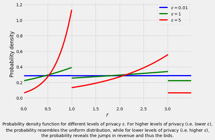
It can be observed that for low values of $\epsilon$ the probability resembles a flat, horizontal curve of the uniform probability, thus the privacy increases. On the contrary, for higher values of $\epsilon$ , the probability curve exponentially reveals the jumps in the revenue, implying less privacy.

4.1) Simulation of the distribution

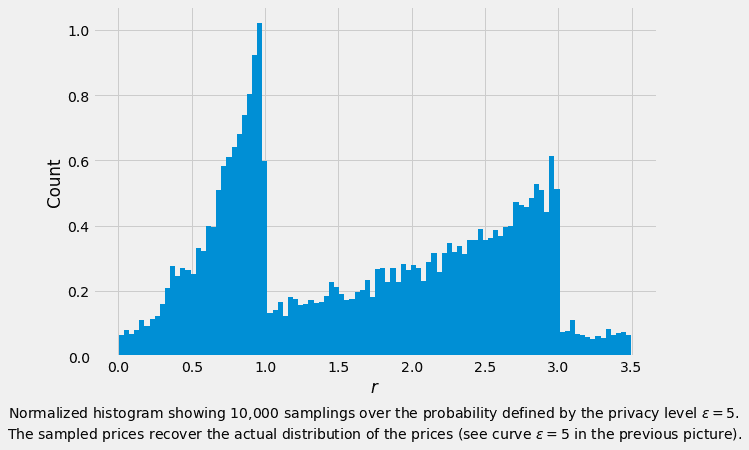
We create a node that contains the true bids and choose to access the data using the exponential mechanism. We repeat the experiment 10,000 times to check that the resulting distribution for the output price matches the one shown earlier.

from shfl.differential_privacy.mechanism import ExponentialMechanism
from shfl.private.node import DataNode

node = DataNode()    # Create a node
node.set_private_data(name="bids", data=np.array(x)) # Store the database x in the node
delta_u = r.max()    # In this specific case, Delta u = max(r)
epsilon = 5          # Set a value for epsilon
size = 10000         # We want to repeat the query this many times

data_access_definition = ExponentialMechanism(u, r, delta_u, epsilon, size)
node.configure_data_access("bids", data_access_definition)
result = node.query("bids")

2022-03-23 13:00:50.983291: W tensorflow/stream_executor/platform/default/dso_loader.cc:64] Could not load dynamic library 'libcudart.so.11.0'; dlerror: libcudart.so.11.0: cannot open shared object file: No such file or directory
2022-03-23 13:00:50.983307: I tensorflow/stream_executor/cuda/cudart_stub.cc:29] Ignore above cudart dlerror if you do not have a GPU set up on your machine.

Now we plot the results, which look like the probability density function defined with $\epsilon$ = 5 as we have anticipated:

fig, ax = plt.subplots(figsize=(9,6))
plt.hist(result, bins = int(round(np.sqrt(len(result)))), density = True)
ax.set_xlabel('$r$')
ax.set_ylabel('Count')
label="Normalized histogram showing 10,000 samplings over the probability defined by the privacy level $\epsilon=5$. \n\
The sampled prices recover the actual distribution of the prices (see curve $\epsilon=5$ in the previous picture)."
ax.text(r.max()/2, -0.25, label, ha='center')

plt.show()

png

4.2) Trade-off between accuracy and privacy

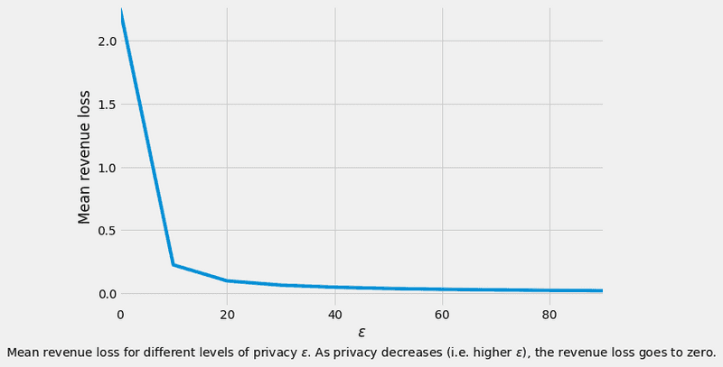
The trade-off between accuracy and privacy can be assessed by computing the mean revenue loss, which is defined as

{\rm {loss}}= |u_{\rm{OPT}}(x) - u(x,r_{\rm{sample}})|

where $u_{\rm{OPT}}(x)$ is the highest possible revenue for a fixed database $x$ , and $u(x,r_{\rm{sample}})$ is the revenue at the sampled price $r_{\rm{sample}}$ .

This is a measure of the loss in utility that we get when using the exponential mechanism compared to the case without any privacy at all.

epsilon_range = np.arange(0.001, 100, 10)
optimum_price = float(r[utility == max(utility)])
optimum_revenue = u(x, [optimum_price])
mean_loss = np.zeros(len(epsilon_range))

for i in range(len(epsilon_range)):
    epsilon = epsilon_range[i]
    node = DataNode()
    node.set_private_data(name="bids", data=np.array(x))
    data_access_definition = ExponentialMechanism(u, r, delta_u, epsilon, size)
    node.configure_data_access("bids", data_access_definition)
    result = node.query("bids")
    mean_loss[i] = np.mean(abs(u(x, result) - optimum_revenue))

The plot below shows that as $\epsilon$ increases (i.e. privacy decreases) the revenue loss goes toward zero, which means higher revenue, but no privacy at all.

fig, ax = plt.subplots(figsize=(9,6))
ax.plot(epsilon_range, mean_loss)
ax.set_xlim([0, max(epsilon_range)])
ax.set_ylim([-0.1, max(mean_loss)])
ax.set_xlabel('$\epsilon$')
ax.set_ylabel('Mean revenue loss')
label="Mean revenue loss for different levels of privacy $\epsilon$. \
As privacy decreases (i.e. higher $\epsilon$), the revenue loss goes to zero."
ax.text(epsilon_range.max()/2, -0.5, label, ha='center')

plt.show()

png

5) Example: randomized response from the exponential mechanism

Consider the case in which $\mathcal R = \{0, 1\}$ and $\mathcal X = \{\text{truly innocent}, \text{truly guilty}\}$ with a utility given by

u(0, 0) = 0\qquad u(1, 0) = 0

u(0, 1) = \beta \qquad u(1, 1) = -\beta

This means that $\Delta u = 2|\beta|$ so $\epsilon = 4\alpha |\beta|$ . For concreteness, in the following we choose $\beta = -1/4$ so that $\epsilon = \alpha$ .

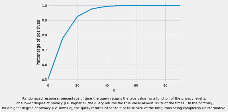
In the figure below we show the percentage of time the query returns the same value as the true value as a function of $\epsilon$ . We observe that this percentage approaches one as the privacy decreases. For $\epsilon=0$ , which provides maximal privacy, the result of the query is completely uninformative since the probability of getting either result is independent of the true value.

Here we define the utility function based on the randomized mechanism:

def u_randomized(x, r):
    '''
    Arguments:
        x: binary number 
        r: array of binaries
    '''
    output = -1/4 * (1 - 2*x) * r
    return output

To use the function above, we need to declare the related variables, and then use the corresponding mechanism so as to declare the data acess definition. In this way, we are applying the randomized response with the exponential mechanism in the queries.

r = np.array([0,1]) # Set the interval of possible outputs r
x = 1               # Set a value for the dataset
delta_u = 1         # We simply set it to one
size = 100000       # We want to repeat the query this many times

epsilon_range = np.arange(0.001, 100, 10)
positives = np.zeros(len(epsilon_range))


for i in range(len(epsilon_range)):
    epsilon = epsilon_range[i]
    node = DataNode()               # Create a node
    node.set_private_data(name="identity", data=np.array(x))  # Store the database x in the node
    data_access_definition = ExponentialMechanism(u_randomized, r, delta_u, epsilon, size)
    node.configure_data_access("identity", data_access_definition)
    result = node.query("identity")
    positives[i] = result.sum() / size

After calculating the results using various epsilon values through various experiments, we plot the percentage of true values returned after a query is performed.

fig, ax = plt.subplots(figsize=(9,6))
ax.plot(epsilon_range, positives)
ax.set_xlim([0, max(epsilon_range)])
ax.set_xlabel('$\epsilon$')
ax.set_ylabel('Percentage of positives')
label="Randomized response: percentage of time the query returns the true value, as a function of the privacy level $\epsilon$.\n\
For a lower degree of privacy (i.e. higher $\epsilon$), the query returns the true value almost 100% of the times. On the contrary, \n\
for a higher degree of privacy (i.e. lower $\epsilon$), the query returns either true or false 50% of the time, thus being completely uninformative."
ax.text(epsilon_range.max()/2, 0.3, label, ha='center')

plt.show()

png

6) Example: Laplace mechanism from the exponential mechanism

We choose the utility function to be $u(x,\,r) = -\left| f(x) - r \right|$ with $r\in\mathbb R$ . By substituting it into the exponential mechanism, we obtain an algorithm with conditional probability

P(r|x; f, \alpha) = \frac{\alpha}{2}e^{-\alpha |f(x) - r|}\,.

In this example we pick $f(x)$ to be the identity. We then only need to define the utility function.

Here we define the utility function for the Laplacian mechanism using the exponential mechanism

def u_laplacian(x, r):
    '''
    Arguments:
        x: float. 
        r: array of reals.
    '''
    output = -np.absolute(x - r)
    return output

And we calculate the experiment using the next values:

# Define some example values:
r = np.arange(-20, 20, 0.001) # Set the interval of possible outputs r
x = 3.5                       # Set a value for the dataset
delta_u = 1                   # We simply set it to one
epsilon = 1                   # Set a value for epsilon
size = 100000                 # We want to repeat the query this many times

node = DataNode()             # Create a node
node.set_private_data(name="identity", data=np.array(x)) # Store the database x in the node

data_access_definition = ExponentialMechanism(u_laplacian, r, delta_u, epsilon, size)
node.configure_data_access("identity", data_access_definition)
result = node.query("identity")

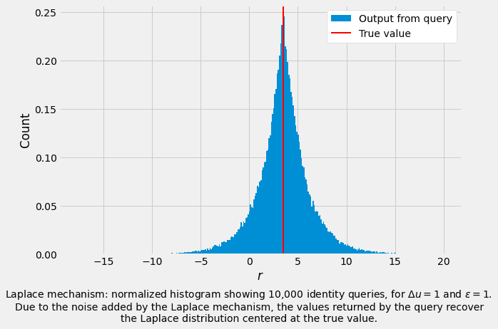
Below, we show a (normalized) histogram of the result of performing the query with Laplace noise, repeatedly. As you can see, it gives us the Laplace distribution centered at the true value $f(x)$ .

fig, ax = plt.subplots(figsize=(9,6))
plt.hist(result, bins = int(round(np.sqrt(len(result)))), density = True, label="Output from query")
plt.axvline(x=x, linewidth=2, color='r', label= "True value")
ax.set_xlabel('$r$')
ax.set_ylabel('Count')
ax. legend(facecolor='white', framealpha=1, frameon=True)
label="Laplace mechanism: normalized histogram showing 10,000 identity queries, for $\Delta u = 1$ and $\epsilon = 1$. \n\
Due to the noise added by the Laplace mechanism, the values returned by the query recover\n\
the Laplace distribution centered at the true value."
ax.text((r.max()+r.min())/2, -0.07, label, ha='center')

plt.show()

png