Federated models: Naïve Bayes (NB)
In this notebook, we explain how you can use a federated learning environment to create a Naïve Bayes model.
The data
First, we load the libraries and we specify gloabl variables for the federated training environment and the model.
import shfl
import numpy as np
import pandas as pd
from shfl.model.tmnb_bin_model import TMNB01Algorithm
from shfl.auxiliar_functions_for_notebooks.functionsFL import *
from shfl.data_base.data_base import WrapLabeledDatabase
from shfl.federated_government.federated_government import FederatedGovernment
from shfl.private.federated_operation import ServerDataNode
from shfl.private.data import DPDataAccessDefinition
from shfl.private.reproducibility import Reproducibility

Reproducibility(567)
2022-04-07 14:18:21.246919: W tensorflow/stream_executor/platform/default/dso_loader.cc:64] Could not load dynamic library 'libcudart.so.11.0'; dlerror: libcudart.so.11.0: cannot open shared object file: No such file or directory
2022-04-07 14:18:21.246939: I tensorflow/stream_executor/cuda/cudart_stub.cc:29] Ignore above cudart dlerror if you do not have a GPU set up on your machine.
<shfl.private.reproducibility.Reproducibility at 0x7fef17893a60>Now we load the data from the file, containing binary features and a final label.
# Load data
df = pd.read_csv("data/database_as_hard_noiid.csv", sep = get_delimiter("data/database_as_hard_noiid.csv"), header=None)
Let's take a look at the data available.
df.head()| 0 | 1 | 2 | 3 | 4 | 5 | 6 | 7 | 8 | 9 | ... | 11 | 12 | 13 | 14 | 15 | 16 | 17 | 18 | 19 | 20 | |
|---|---|---|---|---|---|---|---|---|---|---|---|---|---|---|---|---|---|---|---|---|---|
| 0 | 0 | 0 | 0 | 0 | 0 | 1 | 0 | 1 | 1 | 0 | ... | 0 | 0 | 0 | 0 | 0 | 1 | 0 | 1 | 1 | 0 |
| 1 | 0 | 1 | 1 | 0 | 0 | 0 | 0 | 1 | 0 | 0 | ... | 0 | 1 | 1 | 0 | 1 | 0 | 0 | 0 | 1 | 0 |
| 2 | 0 | 1 | 0 | 0 | 0 | 1 | 1 | 0 | 0 | 1 | ... | 0 | 0 | 1 | 0 | 0 | 0 | 0 | 0 | 0 | 1 |
| 3 | 0 | 0 | 0 | 0 | 0 | 0 | 1 | 0 | 0 | 0 | ... | 0 | 0 | 1 | 0 | 0 | 1 | 0 | 0 | 1 | 0 |
| 4 | 0 | 1 | 0 | 0 | 0 | 0 | 1 | 1 | 0 | 1 | ... | 0 | 1 | 1 | 0 | 0 | 0 | 0 | 0 | 0 | 1 |
5 rows × 21 columns
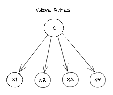
For the NB algorithm, we define the dependencies graph, where features are completely independent from each other.

First of all, we extract the number of features in order to later configure the model.
n_features = len(df.columns) - 1Now, in order to simulate a federated scenario, we need to distribute the data into the nodes. We are using the WrapLabeledDatabase class in order to wrap the data and the labels in a format compatible with the tool. This class also allows us to divide the global data into a global train and test for experimentation purposes.
df = df.to_numpy()
grouped_data = np.delete(df, -1, axis=1)
grouped_labels = df[:, -1]

database = WrapLabeledDatabase(grouped_data,grouped_labels)
_, _, test_data, test_labels = database.load_data()
To finish the distribution, we divide the data in an iid way between the nodes, and we apply an internal split of train and test to locally evaluate their data with the model they are training with.
iid_distribution = shfl.data_distribution.IidDataDistribution(database)
nodes_federation, test_data, test_labels = iid_distribution.get_nodes_federation(num_nodes=5, percent=100)
nodes_federation.split_train_test(0.7);
The model
Next, we define the model_builder() function to create an instance of the NB algorithm.
By the implementation below, we only need to define the number of features of the dataset, previously calculated:
def model_builder():
    model = TMNB01Algorithm(n_features)
    return model
Run the federated learning experiment
After defining the data and the model, we are ready to run our model in a federated configuration. le'ts define the needed components and run the training.
aggregator = shfl.federated_aggregator.FedAvgAggregator()

federated_government = FederatedGovernment(model_builder(), nodes_federation, aggregator)
federated_government.run_rounds(n_rounds=2, test_data=test_data, test_label=test_labels)
Evaluation in round 0:
########################################
Node 0:
-> Global test accuracy:0.9929328621908127
-> Local accuracy:0.9929430214323053
Node 1:
-> Global test accuracy:0.9916574319944801
-> Local accuracy:0.9916361735493988
Node 2:
-> Global test accuracy:0.9963827963284337
-> Local accuracy:0.9957313354821848
Node 3:
-> Global test accuracy:0.9955673573504505
-> Local accuracy:0.9966021955044433
Node 4:
-> Global test accuracy:0.9897547410458528
-> Local accuracy:0.9876295844585765
########################################
Collaborative model test -> 0.994417379304577
Evaluation in round 1:
########################################
Node 0:
-> Global test accuracy:0.9996654609321095
-> Local accuracy:0.9999128768078063
Node 1:
-> Global test accuracy:0.9991009262550442
-> Local accuracy:0.99930301446245
Node 2:
-> Global test accuracy:1.0
-> Local accuracy:1.0
Node 3:
-> Global test accuracy:0.9999790913082568
-> Local accuracy:1.0
Node 4:
-> Global test accuracy:0.9986827524201811
-> Local accuracy:0.9979092255422947
########################################
Collaborative model test -> 1.0