⚠

Please note that these tutorials refer to a deprecated version of the platform. The current version of the platform, which is not publicly available, has a more advanced architecture and provides a wider range of functionalities. These tutorials are only for illustrative purposes and showcase a limited number of the platform’s capabilities.

Horizontal Federated Learning case: Security

In this notebook we present a case where a surveillance company wants to identify who is not wearing face masks on various premises. They have thousands of cameras that can be trained with an AI model to detect if people are wearing masks or not, blocking access to those that are not. This problem is Horizontal Federated Learning since data sets will have the same feature space (same resolution of images) but differ in samples (different images). With the help of Sherpa.ai Federated Learning framework, we design a solution to allow to train the AI model using the data sets of all cameras without sharing any privacy-protected data or images, creating an AI model capable of predicting when people accessing buildings recorded by cameras are not wearing face masks while complying with privacy regulations. The architecture of the solution is:

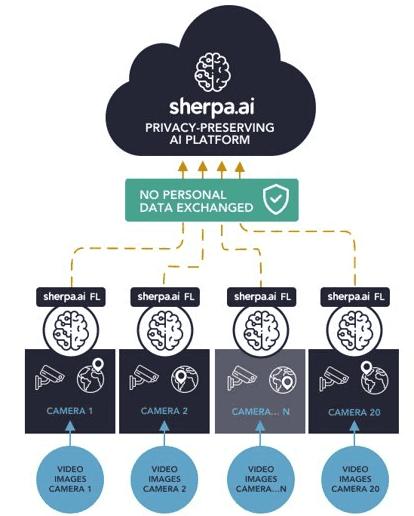
To set up the federated learning experiment we will show the simple steps for loading the dataset and distribute it to a federated network of clients, and we will define the model that will be trained in the federated learning rounds.

Moreover, we will compare a local node's execution with only it's own data, the hipothetical case where all the data is centralized and the federated scenario to check the obtained models' performances against the testing data. Finally, we will further discuss the viability of horizontal Federated Learning.

Once that we have a general overview of our problem, the procedure is the following:

Index

0) Libraries and data

We are going to apply Horizontal Federated Learning to the dataset: https://www.kaggle.com/andrewmvd/face-mask-detection In order to realize this experiment, you should download the dataset in your PC.

Firstly, we load the libraries:

import glob
import os

import cv2
import matplotlib.image as mpimg
import pandas as pd
import tensorflow as tf
import warnings
from tensorflow.keras.regularizers import l2

import shfl
from shfl.auxiliar_functions_for_notebooks.functionsFL import *
from shfl.data_base.data_base import WrapLabeledDatabase
from shfl.private.reproducibility import Reproducibility

plt.style.use('seaborn')
warnings.filterwarnings('ignore')
Reproducibility(567)

2022-04-25 11:59:31.711140: W tensorflow/stream_executor/platform/default/dso_loader.cc:64] Could not load dynamic library 'libcudart.so.11.0'; dlerror: libcudart.so.11.0: cannot open shared object file: No such file or directory; LD_LIBRARY_PATH: /home/x.sarrionaindia/Documentos/virtual/virtual/lib/python3.8/site-packages/cv2/../../lib64:
2022-04-25 11:59:31.711174: I tensorflow/stream_executor/cuda/cudart_stub.cc:29] Ignore above cudart dlerror if you do not have a GPU set up on your machine.





<shfl.private.reproducibility.Reproducibility at 0x7f7901095fd0>

We have to load the images in this notebook. The data is splited in two folders with_mask and without_mask:

base_dir = './data_FaceMask/'

with_mask_dir = os.path.join(base_dir, 'with_mask/')
without_mask_dir = os.path.join(base_dir, 'without_mask/')

But first let's take a look of how are these images:images:

nrows = 8
ncols = 8
pic_index = 0 # Index for iterating over images
fig = plt.gcf()
fig.set_size_inches(ncols*8, nrows*8)
with_mask_fnames = os.listdir( with_mask_dir )
without_mask_fnames = os.listdir( without_mask_dir)


with_mask_pix= [os.path.join(with_mask_dir , fname) 
                for fname in with_mask_fnames[ pic_index:pic_index+8]
               ]

without_mask_pix=  [os.path.join(without_mask_dir, fname) 
                for fname in without_mask_fnames[ pic_index:pic_index+8]
               ]
for i, img_path in enumerate(with_mask_pix+without_mask_pix):
  # Set up subplot; subplot indices start at 1
    sp = plt.subplot(nrows, ncols, i+1)
    sp.axis('ON')  # Show the gridlines

    img = mpimg.imread(img_path)
    plt.imshow(img)

plt.show()

png

As we can see, the sizes of the images are different, so we will have to reshape the images to the same size if we want to apply Horizontal Federated Learning.

1) Preprocessing

We load the names of the files:

with_mask_dataset=sorted(glob.glob("./data_FaceMask/with_mask/*.jpg"))
without_mask_dataset=sorted(glob.glob("./data_FaceMask/without_mask/*.jpg"))

In this example, we are going to give a label 0 if it have a mask and 1 if it has not a mask.

df_withmask = pd.DataFrame(with_mask_dataset, columns = ['filepath'])
df_withmask["label"]=0

df_withmask.head()

	filepath	label
0	./data_FaceMask/with_mask/with_mask_1.jpg	0
1	./data_FaceMask/with_mask/with_mask_10.jpg	0
2	./data_FaceMask/with_mask/with_mask_100.jpg	0
3	./data_FaceMask/with_mask/with_mask_1000.jpg	0
4	./data_FaceMask/with_mask/with_mask_1001.jpg	0

df_withoutmask = pd.DataFrame(without_mask_dataset, columns = ['filepath'])
df_withoutmask["label"]=1

df_withoutmask.head()

	filepath	label
0	./data_FaceMask/without_mask/without_mask_1.jpg	1
1	./data_FaceMask/without_mask/without_mask_10.jpg	1
2	./data_FaceMask/without_mask/without_mask_100.jpg	1
3	./data_FaceMask/without_mask/without_mask_1000...	1
4	./data_FaceMask/without_mask/without_mask_1001...	1

Now we join all the data to have pictures with mask and without mask and we will shuffle the rows.

WARNING: We are going to do this because later is going to be splited in different nodes. In a real-world scenario, the images would already be in the nodes.

df_centralized = df_withmask.append(pd.DataFrame(data = df_withoutmask), ignore_index=True)

df_centralized = df_centralized.sample(frac=1).reset_index(drop=True)

df_centralized is then the non-privacy case where all the images are alocated together.

We have the directories, but we need the data, so we will use the cv2 library to translate the files to arrays:

Note, cv2 can be installed with the command: pip install opencv-python)

data_array=[]
for i in range(len(df_centralized.filepath)):
    data_array.append(cv2.imread((df_centralized.filepath[i])))

If we want to use the same model (we are in a horizontal scenario), the dimension of all the images has to be the same. We have already check that the dimension of the images are differents

To solve that, we will reshape the images in each node to a dimension of (64,64,3), both in train and test.

for i in range(len(df_centralized.filepath)):
    data_array[i]=cv2.resize(data_array[i], (64,64))

Now we convert the data to array:

data=np.array(data_array)

labels=df_centralized["label"].to_numpy()

And we transform the output variable in order to work with a Neural Network.

labels=np.eye(2)[labels]

Thanks to the function WrapLabeledDatabase, we generate the processed database and we are ready to split it among the nodes:

database=WrapLabeledDatabase(data,labels)

Before training the model, we have to select which data is going to be sent to the nodes. This way, we will send the train_data and train_labels to the federated nodes.

The test_data and test_labels correspond to a data to check how different the federated model behaves in comparison with the local one and the centralized one. WARNING: This can not happen in a real world-scenario, since different parties can not share any percent of their data. As this notebook is done for educational purposes, we take a percent of the total data (20%) that will be use to stablish a benchmark.

train_data, train_labels, test_data, test_labels = database.load_data()

iid_distribution = shfl.data_distribution.IidDataDistribution(database)


nodes_federation, test_data, test_labels = iid_distribution.get_nodes_federation(num_nodes=20, percent=100)

That's it! We have created federated data from the Face Mask dataset using 10 nodes with all the avaliable data (i.e, the 100 percent of the data). This means that all the data is distributed in the 20 nodes. Note that the data is IID distributed.

Before running the algorithm, we want to apply a transformation to the data. A good practice is to define a federated operation that will ensure that the transformation is applied to the federated data in all the client nodes. We want to normalize the data, so we define the following function:

def normalize_data(data):
    data.data = (data.data / 255)

This is done to have the range of data from 0 to 1, instead of [0,255]

nodes_federation.apply_data_transformation(normalize_data);

And we do the same with the test data:

test_data=test_data/255

2) Run the experiment

The model that we are going to use to develop our experiment is the next one:

def facemask_deeplearning_model_builder():
    """"
    Implement a Deep Learning Model for the dataset of FaceMask
    (see https://www.kaggle.com/omkargurav/face-mask-dataset)
    The metrics will be the log-loss and the accuracy.
    """
    model = tf.keras.models.Sequential()
    model.add(tf.keras.layers.Conv2D(32, kernel_size=(3, 3), activation='relu', input_shape=(64, 64, 3)))
    model.add(tf.keras.layers.MaxPooling2D(2, 2))
    model.add(tf.keras.layers.Conv2D(64, kernel_size=(3, 3), activation='relu'))
    model.add(tf.keras.layers.MaxPooling2D(2, 2))
    model.add(tf.keras.layers.Conv2D(128, kernel_size=(3, 3), activation='relu'))
    model.add(tf.keras.layers.MaxPooling2D(2, 2))
    model.add(tf.keras.layers.Conv2D(128, kernel_size=(3, 3), activation='relu', kernel_regularizer=l2(0.0005)))
    model.add(tf.keras.layers.MaxPooling2D(2, 2))
    model.add(tf.keras.layers.Flatten())
    model.add(tf.keras.layers.Dropout(0.5))
    model.add(tf.keras.layers.Dense(512, activation='relu'))
    model.add(tf.keras.layers.Dense(2, activation='softmax'))

    loss = tf.keras.losses.CategoricalCrossentropy()
    optimizer = tf.keras.optimizers.Adam()
    metrics = [tf.keras.metrics.categorical_accuracy]
    epochs = 1 
    batch_size = 32

    return shfl.model.DeepLearningModel(model=model, loss=loss, optimizer=optimizer,
                                        batch_size=batch_size, epochs=epochs, metrics=metrics)

2.1) Federated

aggregator = shfl.federated_aggregator.FedAvgAggregator()
federated_government = shfl.federated_government.FederatedGovernment(facemask_deeplearning_model_builder(), nodes_federation
                                                                     , aggregator
                                                                    )

2022-04-25 12:00:00.615283: W tensorflow/stream_executor/platform/default/dso_loader.cc:64] Could not load dynamic library 'libcuda.so.1'; dlerror: libcuda.so.1: cannot open shared object file: No such file or directory; LD_LIBRARY_PATH: /home/x.sarrionaindia/Documentos/virtual/virtual/lib/python3.8/site-packages/cv2/../../lib64:
2022-04-25 12:00:00.615310: W tensorflow/stream_executor/cuda/cuda_driver.cc:269] failed call to cuInit: UNKNOWN ERROR (303)
2022-04-25 12:00:00.615327: I tensorflow/stream_executor/cuda/cuda_diagnostics.cc:156] kernel driver does not appear to be running on this host (SH-083-WS): /proc/driver/nvidia/version does not exist
2022-04-25 12:00:00.615526: I tensorflow/core/platform/cpu_feature_guard.cc:151] This TensorFlow binary is optimized with oneAPI Deep Neural Network Library (oneDNN) to use the following CPU instructions in performance-critical operations:  AVX2 FMA
To enable them in other operations, rebuild TensorFlow with the appropriate compiler flags.

federated_government.run_rounds(10, test_data, test_labels)

WARNING:tensorflow:5 out of the last 9 calls to <function Model.make_test_function.<locals>.test_function at 0x7f78705bc5e0> triggered tf.function retracing. Tracing is expensive and the excessive number of tracings could be due to (1) creating @tf.function repeatedly in a loop, (2) passing tensors with different shapes, (3) passing Python objects instead of tensors. For (1), please define your @tf.function outside of the loop. For (2), @tf.function has experimental_relax_shapes=True option that relaxes argument shapes that can avoid unnecessary retracing. For (3), please refer to https://www.tensorflow.org/guide/function#controlling_retracing and https://www.tensorflow.org/api_docs/python/tf/function for  more details.
WARNING:tensorflow:6 out of the last 11 calls to <function Model.make_test_function.<locals>.test_function at 0x7f78706e23a0> triggered tf.function retracing. Tracing is expensive and the excessive number of tracings could be due to (1) creating @tf.function repeatedly in a loop, (2) passing tensors with different shapes, (3) passing Python objects instead of tensors. For (1), please define your @tf.function outside of the loop. For (2), @tf.function has experimental_relax_shapes=True option that relaxes argument shapes that can avoid unnecessary retracing. For (3), please refer to https://www.tensorflow.org/guide/function#controlling_retracing and https://www.tensorflow.org/api_docs/python/tf/function for  more details.
Evaluation in round 0:

Collaborative model test -> loss: 0.7292401194572449  categorical_accuracy: 0.7888815402984619  

Evaluation in round 1:

Collaborative model test -> loss: 0.6105746626853943  categorical_accuracy: 0.8312376141548157  

Evaluation in round 2:

Collaborative model test -> loss: 0.44488829374313354  categorical_accuracy: 0.84315025806427  

Evaluation in round 3:

Collaborative model test -> loss: 0.3967798948287964  categorical_accuracy: 0.8471211194992065  

Evaluation in round 4:

Collaborative model test -> loss: 0.35977083444595337  categorical_accuracy: 0.8649900555610657  

Evaluation in round 5:

Collaborative model test -> loss: 0.3331293761730194  categorical_accuracy: 0.8755790591239929  

Evaluation in round 6:

Collaborative model test -> loss: 0.3080635666847229  categorical_accuracy: 0.8788881301879883  

Evaluation in round 7:

Collaborative model test -> loss: 0.29005342721939087  categorical_accuracy: 0.8874917030334473  

Evaluation in round 8:

Collaborative model test -> loss: 0.27629202604293823  categorical_accuracy: 0.8894771933555603  

Evaluation in round 9:

Collaborative model test -> loss: 0.26078900694847107  categorical_accuracy: 0.894109845161438

We have obtained the accuracy of the federated model, but now we are going to extract the predictions to obtain the ROC-AUC curve, since we will then be able to compare the different results.

federated_model = federated_government._server._model
predictions_fed = federated_model.predict(test_data)

accuracy_federated_20=accuracy(predictions_fed, test_labels)
accuracy_federated_20

0.8941098610191925

plot_roc(predictions_fed, test_labels)

png

2.2) Local (Data with only one camera)

For the local test, we implemented a method to obtain the node's data experimentally. However, THIS IS NOT APPLICABLE IN A REAL CASE OR IN THE PLATFORM AND IT IS MADE FOR TESTING PURPOSES ONLY. All of these notebooks are made with an experimental implementation of the code where security measures are bypassed for explainability reasons. We take, for example, the data of the first node the local benchmark.

for i in nodes_federation[0]._private_data:
    local_data = nodes_federation[0]._private_data[i].data
    local_label = nodes_federation[0]._private_data[i].label

model_loc = facemask_deeplearning_model_builder()
model_loc.train(local_data, local_label)

predictions_loc = model_loc.predict(test_data)

accuracy_local_20=accuracy(predictions_loc, test_labels)
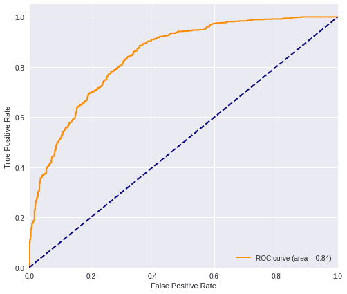
accuracy_local_20

0.7564526803441429

plot_roc(predictions_loc, test_labels)

png

2.3) Centralized (Data joined but with any privacy)

This correspond to the case of Traditional Machine Learning which requires all the data to be gathered in one single place. In practice, this is often forbidden by privacy regulations.

train_data_centralized = train_data/255

model_cent = facemask_deeplearning_model_builder()
model_cent.train(train_data_centralized, train_labels)

predictions_cent = model_cent.predict(test_data)

accuracy_centralized=accuracy(predictions_cent, test_labels)
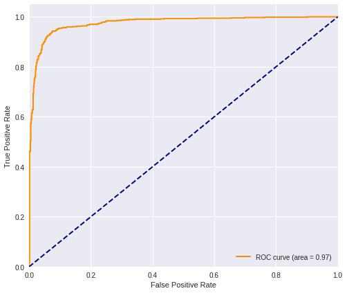
accuracy_centralized

0.8881535407015222

plot_roc(predictions_cent, test_labels)

png

2.4) Comparison

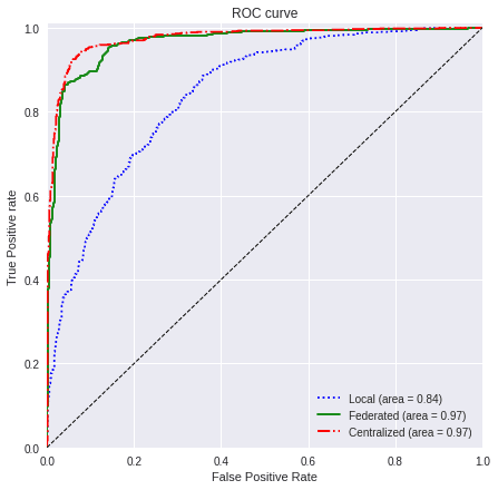
We are going now to use the ROC curve and the F1-Score to compare the different results that we have obtained. We will then be able to understand the improvements that using federated learning brings in this scenario.

values=[predictions_loc, predictions_fed, predictions_cent]
titles=['Local', 'Federated', 'Centralized']
colors=['blue', 'green', 'red']
linestyle=[':','-','-.']

plot_all_roc_curves(test_labels, values, titles, colors, linestyle)

png

test_labels

array([[1., 0.],
       [1., 0.],
       [1., 0.],
       ...,
       [0., 1.],
       [0., 1.],
       [0., 1.]])

predictions_loc

array([[0.49995548, 0.5000445 ],
       [0.50844854, 0.4915514 ],
       [0.50593996, 0.49406007],
       ...,
       [0.49678254, 0.5032174 ],
       [0.50839025, 0.49160978],
       [0.49714205, 0.502858  ]], dtype=float32)

score_loc_f1_20 = f1(test_labels, predictions_loc)
score_fed_f1_20 = f1(test_labels, predictions_fed)
score_cent_f1_20 = f1(test_labels, predictions_cent)

f1scores=[round(score_loc_f1_20, 4),
        round(score_fed_f1_20, 4),
        round(score_cent_f1_20, 4)]

titles=['Local',
        'Federated',
        'Centralized']

colors=['blue',
        'green',
        'red']

plot_all_metric(f1scores, 'F1-Score', titles, colors)

png

Taking into account the results of the ROC AUC and the F1-Score, we can assure that using a Federated Learning scenario in this problem is really convenient, since the improvement with respect to the local is huge (an improvement of 0.1 of AUC and an improvement of 0.546 in F1-Score).

Let's see now the accuracies of the different cases:

accuracies = [round(accuracy_local_20,4), round(accuracy_federated_20,4), round(accuracy_centralized,4)]
plot_all_metric(accuracies, 'Accuracy', titles, colors)

png

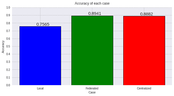
We have to notice that we get a result using federated learning as good as the centralized case. Getting more accuracy than the centralized case does not mean that federated learning improves the results. This small difference can be due to random factors as the initialization of the params or the convergence of the loss function. In any case, we can reach to the conclusion that federated learning is an excellent tool to improve the results in a privacy-preserving manner in comparison with a local scenario.

2.5) Changing the number of cameras/nodes

In the case that we have presented in the preceding sections, we have supposed that we have few cameras with a lot of data in each of them. We can now generate an opposite scenario, where we have a lot of cameras but with few data. Said that, let's see what happens if we increase the number of nodes to a huge one (200 cameras), but keeping the same amount of data. This will mean that the cameras will have few data in each of them.

nodes_federation_2, test_data, test_labels = iid_distribution.get_nodes_federation(num_nodes=200, percent=100)
test_data = test_data/255
nodes_federation_2.apply_data_transformation(normalize_data);
aggregator = shfl.federated_aggregator.FedAvgAggregator()
federated_government_2 = shfl.federated_government.FederatedGovernment(facemask_deeplearning_model_builder(), nodes_federation_2
                                                                     , aggregator
                                                                    )
federated_government_2.run_rounds(10, test_data, test_labels)

WARNING:tensorflow:5 out of the last 156 calls to <function Model.make_train_function.<locals>.train_function at 0x7f78003cb8b0> triggered tf.function retracing. Tracing is expensive and the excessive number of tracings could be due to (1) creating @tf.function repeatedly in a loop, (2) passing tensors with different shapes, (3) passing Python objects instead of tensors. For (1), please define your @tf.function outside of the loop. For (2), @tf.function has experimental_relax_shapes=True option that relaxes argument shapes that can avoid unnecessary retracing. For (3), please refer to https://www.tensorflow.org/guide/function#controlling_retracing and https://www.tensorflow.org/api_docs/python/tf/function for  more details.
WARNING:tensorflow:6 out of the last 157 calls to <function Model.make_train_function.<locals>.train_function at 0x7f780020c5e0> triggered tf.function retracing. Tracing is expensive and the excessive number of tracings could be due to (1) creating @tf.function repeatedly in a loop, (2) passing tensors with different shapes, (3) passing Python objects instead of tensors. For (1), please define your @tf.function outside of the loop. For (2), @tf.function has experimental_relax_shapes=True option that relaxes argument shapes that can avoid unnecessary retracing. For (3), please refer to https://www.tensorflow.org/guide/function#controlling_retracing and https://www.tensorflow.org/api_docs/python/tf/function for  more details.
Evaluation in round 0:

Collaborative model test -> loss: 0.7483205795288086  categorical_accuracy: 0.6499007344245911  

Evaluation in round 1:

Collaborative model test -> loss: 0.7399173378944397  categorical_accuracy: 0.675711452960968  

Evaluation in round 2:

Collaborative model test -> loss: 0.7301623225212097  categorical_accuracy: 0.6379880905151367  

Evaluation in round 3:

Collaborative model test -> loss: 0.7179173827171326  categorical_accuracy: 0.6657842397689819  

Evaluation in round 4:

Collaborative model test -> loss: 0.7008394598960876  categorical_accuracy: 0.7557908892631531  

Evaluation in round 5:

Collaborative model test -> loss: 0.6787611842155457  categorical_accuracy: 0.8371939063072205  

Evaluation in round 6:

Collaborative model test -> loss: 0.650204062461853  categorical_accuracy: 0.8484447598457336  

Evaluation in round 7:

Collaborative model test -> loss: 0.6189337372779846  categorical_accuracy: 0.8093977570533752  

Evaluation in round 8:

Collaborative model test -> loss: 0.5858006477355957  categorical_accuracy: 0.8093977570533752  

Evaluation in round 9:

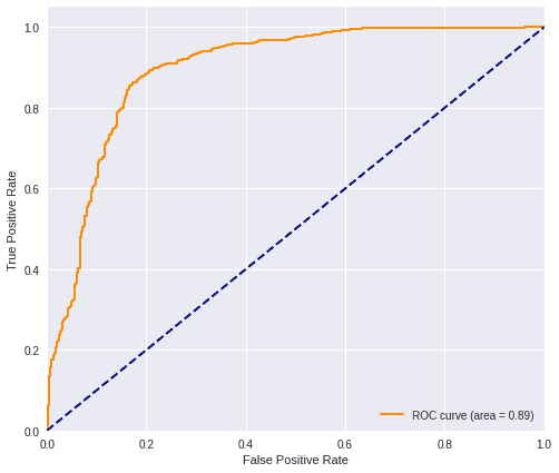
Collaborative model test -> loss: 0.5436283349990845  categorical_accuracy: 0.84315025806427

The ROC curve for the federated scenario is:

federated_model_2 = federated_government_2._server._model
predictions_fed_2 = federated_model_2.predict(test_data)
plot_roc(predictions_fed_2, test_labels)

png

accuracy_federated_200=accuracy(predictions_fed_2, test_labels)
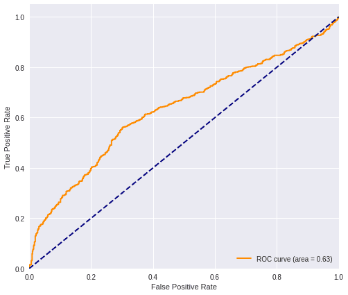
accuracy_federated_200

0.8431502316346791

Now we do an idem for the local case. Remember that in this case, a camera will have a huge amount of data.

for i in nodes_federation_2[0]._private_data:
    local_data_2 = nodes_federation_2[0]._private_data[i].data
    local_label_2 = nodes_federation_2[0]._private_data[i].label
    
model_loc_2 = facemask_deeplearning_model_builder()
model_loc_2.train(local_data_2, local_label_2)

predictions_loc_2 = model_loc_2.predict(test_data)

accuracy_local_200=accuracy(predictions_loc_2, test_labels)
accuracy_local_200

0.48974189278623426

plot_roc(predictions_loc_2, test_labels)

png

The centralized case is exactly the same, since it has all the images, so we do not have to calculate it again.

It is interesting to compare all the different ROC AUC that we have seen:

roc_auc_different_number_of_nodes(test_labels,
                                  predictions_fed, predictions_loc,
                                  predictions_fed_2, predictions_loc_2, predictions_cent)

png

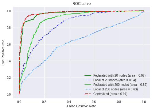
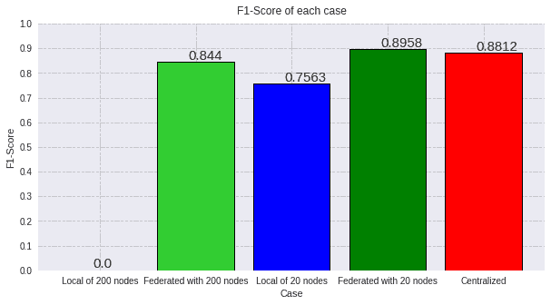
Bearing in mind the fact that here we have 200 nodes with few images, this result demonstrates that federated learning is a really powerful tool to work with data silos preserving the privacy. Said so, we can observe that the federated scenario improves the metric of the local cases measuring both the accuracy and the F1-score:

F1-Score:

score_loc_f1_200 = f1(test_labels, predictions_loc_2)
score_fed_f1_200 = f1(test_labels, predictions_fed_2)
score_cent_f1_200 = f1(test_labels, predictions_cent)

values=[round(score_loc_f1_200, 4),
        round(score_fed_f1_200, 4),
        round(score_loc_f1_20, 4),
        round(score_fed_f1_20, 4),
        round(score_cent_f1_20, 4)]

titles=['Local of 200 nodes',
        'Federated with 200 nodes',
        'Local of 20 nodes',
        'Federated with 20 nodes',
        'Centralized']

colors=['dodgerblue',
        'limegreen', 
        'blue',
        'green',
        'red']

plot_all_metric(values,'F1-Score', titles, colors)

png

Accuracy:

values=[round(accuracy_local_200, 4),
        round(accuracy_federated_200, 4),
        round(accuracy_local_20, 4),
        round(accuracy_federated_20, 4),
        round(accuracy_centralized, 4)]


plot_all_metric(values,'Accuracy', titles, colors)

png

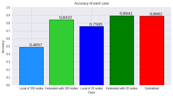
The information that we can obtain with these graphs, is that both local cases performs really bad, even though the one with 20 nodes have a really big amount of data. On the other hand, the federated cases have really good results, and the case with 20 nodes notably improves with respect to the one of 200 nodes. The improve is so remarkable that is really similar to the centralized case that has no privacy constrictions. This leads us to the conclusion that federated learning is always a good option to deal with data silos.

Another conclusion that we can extract, is that we can assure that the less number of nodes, the closer we are from the centralized case. In fact, in the extreme case where the number of nodes is equal to one, local = federated = centralized.