Using Differential Privacy in an Horizontal Federated Learning case

In this notebook we provide a example of how Differential Privacy is added in the Sherpa's platform and the effects it has on the whole process. To set up the federated learning experiment we will replicate the same process of classifying the EMNIST dataset using horizontal Federated Learning in order to train a deep learning model.

This first part is a replica of the horizontal Federated Learning case using the EMNIST dataset, following the same steps. The descriptions of each of the parts are brief, as it main focus is on the Differential Privacy part.

Once that we have a general overview of our problem, the procedure is the following:

Index

We are going to use the EMNIST dataset: the framework provides some functions to load the Emnist digits dataset.

0) Libraries and data

import matplotlib.pyplot as plt
import numpy as np
import shfl
import tensorflow as tf
from shfl.auxiliar_functions_for_notebooks.functionsFL import *
from shfl.differential_privacy import LaplaceMechanism
from shfl.differential_privacy.norm import L1SensitivityNorm
from shfl.differential_privacy.sensitivity_sampler import SensitivitySampler
from shfl.model.functions_for_models import get_trainable_model_sample
from shfl.model.deep_learning_model import DeepLearningModel
from sklearn.metrics import f1_score
from sklearn.metrics import roc_curve, roc_auc_score, auc

plt.style.use('seaborn')


database = shfl.data_base.Emnist()
train_data, train_labels, test_data, test_labels = database.load_data()

2022-04-25 12:19:11.778629: W tensorflow/stream_executor/platform/default/dso_loader.cc:64] Could not load dynamic library 'libcudart.so.11.0'; dlerror: libcudart.so.11.0: cannot open shared object file: No such file or directory
2022-04-25 12:19:11.778661: I tensorflow/stream_executor/cuda/cudart_stub.cc:29] Ignore above cudart dlerror if you do not have a GPU set up on your machine.```

Let's inspect some properties of the loaded data.

print(len(train_data))
print(len(test_data))
print(type(train_data[0]))
print(train_data[0].shape)
print(test_data[0].shape)

240000
40000
<class 'numpy.ndarray'>
(28, 28)
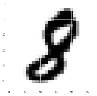
(28, 28)

So, as we have seen, our dataset is composed of a set of matrices that are 28 by 28. Before starting with the federated scenario, we can take a look at a sample of the training data.

plt.imshow(train_data[0])

<matplotlib.image.AxesImage at 0x7f877899ebe0>

1) Prepare the data and the models for the horizontal federated learning scenario preserving the privacy

We are going to simulate a federated learning scenario with a set of client nodes containing private data, and a central server that will be responsible for coordinating the different clients. In order to do that, we are distributing the data independently and identically, in other words, every node is having approximately the same amount of data following the same distribution.

iid_distribution = shfl.data_distribution.IidDataDistribution(database)
nodes_federation, test_data, test_labels = iid_distribution.get_nodes_federation(num_nodes=5, percent=10)

That's it! We have created federated data from the Emnist dataset using 5 nodes and 10 percent of the available data.

A federated learning algorithm is defined by a machine learning model, locally deployed in each node, that learns from the respective node's private data and an aggregating mechanism to _aggregate the different model parameters uploaded by the client nodes to a central node. In this example, we will use a deep learning model using Keras to build it.

Instead of returning the direct model, we will wrap it in another class and return it to extend the functionality to be able to implement Differential Privacy later.

def model_builder():
    model = tf.keras.models.Sequential()
    model.add(tf.keras.layers.Conv2D(32, kernel_size=(3, 3), padding='same', activation='relu', strides=1, input_shape=(28, 28,1)))
    model.add(tf.keras.layers.MaxPooling2D(pool_size=2, strides=2, padding='valid'))
    model.add(tf.keras.layers.Dropout(0.4))
    model.add(tf.keras.layers.Conv2D(32, kernel_size=(3, 3), padding='same', activation='relu', strides=1))
    model.add(tf.keras.layers.MaxPooling2D(pool_size=2, strides=2, padding='valid'))
    model.add(tf.keras.layers.Dropout(0.3))
    model.add(tf.keras.layers.Flatten())
    model.add(tf.keras.layers.Dense(128, activation='relu'))
    model.add(tf.keras.layers.Dropout(0.1))
    model.add(tf.keras.layers.Dense(64, activation='relu'))
    model.add(tf.keras.layers.Dense(10, activation='softmax'))

    loss = tf.keras.losses.CategoricalCrossentropy()
    optimizer = tf.keras.optimizers.RMSprop()
    metrics = [tf.keras.metrics.categorical_accuracy]


    return get_trainable_model_sample(DeepLearningModel(model=model, loss=loss, optimizer=optimizer, metrics=metrics))

In addition, we want to normalize the data. The EMNIST dataset is composed by images, and each of the pixels value range between 0 - 255, so in order to normalize the data and set it to a range between 0 - 1, the rescaling is done by dividing the original value with 255.

Moreover, depending on the image type and the model framework, there are sligth adaptations that need to be done. In this case, the image data needs to be reshaped to indicate the model which are the dimensions and the color channel.

Finally, the transforming operations need to be implemented on both trainig data and test data.

nodes_federation.apply_data_transformation(normalize_data_image);
nodes_federation.apply_data_transformation(reshape_data_tf);
nodes_federation.apply_data_transformation(cast_to_float);

test_data = np.reshape(test_data, (test_data.shape[0], test_data.shape[1], test_data.shape[2],1))
test_data=test_data/255

In the following piece of code, we define the federated aggregation mechanism. Moreover, we define the federated government based on the Keras learning model, the federated data, and the aggregation mechanism.

aggregator = shfl.federated_aggregator.FedAvgAggregator()
federated_government = shfl.federated_government.FederatedGovernment(model_builder(), nodes_federation, aggregator)

2022-04-25 12:19:15.349230: W tensorflow/stream_executor/platform/default/dso_loader.cc:64] Could not load dynamic library 'libcuda.so.1'; dlerror: libcuda.so.1: cannot open shared object file: No such file or directory
2022-04-25 12:19:15.349252: W tensorflow/stream_executor/cuda/cuda_driver.cc:269] failed call to cuInit: UNKNOWN ERROR (303)
2022-04-25 12:19:15.349272: I tensorflow/stream_executor/cuda/cuda_diagnostics.cc:156] kernel driver does not appear to be running on this host (SH-083-WS): /proc/driver/nvidia/version does not exist
2022-04-25 12:19:15.349416: I tensorflow/core/platform/cpu_feature_guard.cc:151] This TensorFlow binary is optimized with oneAPI Deep Neural Network Library (oneDNN) to use the following CPU instructions in performance-critical operations:  AVX2 FMA
To enable them in other operations, rebuild TensorFlow with the appropriate compiler flags.

2) Run the federated learning experiment

We are now ready to execute our horizontal Federated Learning algorithm.

federated_government.run_rounds(5, test_data, test_labels)

Evaluation in round 0:

Collaborative model test -> loss: 0.50938880443573  categorical_accuracy: 0.8656749725341797

Evaluation in round 1:

Collaborative model test -> loss: 0.20250864326953888  categorical_accuracy: 0.9422749876976013

Evaluation in round 2:

Collaborative model test -> loss: 0.1457526981830597  categorical_accuracy: 0.9581249952316284

Evaluation in round 3:

Collaborative model test -> loss: 0.11536990106105804  categorical_accuracy: 0.9660249948501587

Evaluation in round 4:

Collaborative model test -> loss: 0.09375324845314026  categorical_accuracy: 0.9715999960899353

3) Adding differential privacy

Differential Privacy is a statistical technique to provide data aggregations, while avoiding the leakage of individual data records. This technique ensures that malicious agents intervening in the communication of local parameters cannot trace this information back to the data sources, adding an additional layer of data privacy.

There are few steps towards adding this privacy layer, as it needs to be properly adapted to the data. First the sensitivity of the data, then the noise mechanism and finally the parameters of the mechanism, also called the privacy parameter or privacy budget.

3.1) Calculating sensitivity

Roughly speaking, the sensitivity of a function reflects the amount the function’s output will change when its input changes. Notice that, in general, it is not possible to compute the expected value (or any other statistic) of $\Delta f$ exactly. However, the statistics can be estimated using a sampling procedure (see Rubinstein 2017). That is, instead of computing the global sensitivity $\Delta f$ analytically, we compute an empirical estimation of it by sampling over the dataset.

As data composed by images is computationally more expensive to use, we will define a small sample of 20 to calculate the sensitivity.

size = 20

sampling_data = test_data[-size:, ]
sampling_labels = test_labels[-size:, ]

sampling_tuple = (sampling_data,sampling_labels) #tupla

Now, the sample needs to vary with a single distinct image to see how much the output changes. To select a completely random image, we create a uniform probability distribution that will return a similar dataset each time with a different image.

class UniformDistribution(shfl.differential_privacy.ProbabilityDistribution):
    """
    Implement Uniform sampling over the data
    """
    def __init__(self, sample_data):
        self._sample_data = sample_data

    def sample(self, sample_size):
        row_indices = np.random.randint(low=0, high=len(self._sample_data), size=sample_size, dtype='l')
        return (self._sample_data[0][row_indices, :],self._sample_data[1][row_indices, :])

Now that we have all the components to calculate the sensitivity, the sample_sensitivity method will do all the work.

distribution = UniformDistribution(sampling_tuple)

sampler = SensitivitySampler()
n_data_size = 20

max_sensitivity, mean_sensitivity = sampler.sample_sensitivity(
    model_builder(),
    L1SensitivityNorm(), distribution, n_data_size=n_data_size, gamma=0.05)
print("Max sensitivity from sampling: " + str(max_sensitivity))
print("Mean sensitivity from sampling: " + str(mean_sensitivity))

Max sensitivity from sampling: [0.71116817, 0.07792654, 21.385593, 0.09090796, 279.41705, 0.19839986, 10.361249, 0.10681815, 1.1904168, 0.02018311]
Mean sensitivity from sampling: [0.003688997, 0.0005106189, 0.07856818, 0.00038431576, 0.98711646, 0.00064655597, 0.045678724, 0.0003134581, 0.0035663345, 3.2046213e-05]```

3.2) Adding the noise mechanism: trade-off between accuracy and privacy

The noise mechanism is one of the principal components of Differential Privacy. In this notebook, we are using the Laplace distribution to implement it on the model's weight.

The Laplace mechanism consists in adding random noise taken from a Laplace distribution to the data we are targeting. This is commonly used with real numbers, and the bigger the dataset is, the more privacy it gives.

This mechanism satisfies the ε-differential privacy property. This asserts that for all pairs of adjacent databases and all outputs, an adversary cannot distinguish which is the true database on the basis of observing the output. In Differential Privacy, ε is a metric of privacy loss at a differential change in data. A smaller ε will yield better privacy but less accurate response, and viceversa.

Adjusting Differential Privacy enables controlling the amount of noise added to the masking process, allowing the user to choose the exact balance between accuracy and privacy to adapt to the needs of any scenario.

params_access_definition = LaplaceMechanism(sensitivity=mean_sensitivity, epsilon=0.1)

nodes_federation.configure_model_params_access(params_access_definition);

4) Run the federated learning experiment with differential privacy

We are now ready to execute our federated learning algorithm but adding differential privacy on the weights of the local models. When the model weights are shared, they will contain controlled noise, adding a layer of masking that prevents other from tracing back the information, mantaining privacy.

In order to compare the effect of ε in the model performance, we are computing various trainings with distinct values. This means that we are going to change the privacy budget. As the outputs of the trainings are very repetitive, they are going to be ommited and only the first one is going to be shown.

4.1) Training with ε = 0.1

federated_government_dp = shfl.federated_government.FederatedGovernment(
    model_builder(), nodes_federation, aggregator)

federated_government_dp.run_rounds(5, test_data, test_labels)

Evaluation in round 0:

Collaborative model test -> loss: 752.6538696289062  categorical_accuracy: 0.10395000129938126

Evaluation in round 1:

Collaborative model test -> loss: 164.77978515625  categorical_accuracy: 0.14569999277591705

Evaluation in round 2:

Collaborative model test -> loss: 27.08574676513672  categorical_accuracy: 0.12242499738931656

Evaluation in round 3:

Collaborative model test -> loss: 6.61383056640625  categorical_accuracy: 0.1114249974489212

Evaluation in round 4:

Collaborative model test -> loss: 20.337047576904297  categorical_accuracy: 0.08237499743700027

4.2) Training with ε = 1

We need to implement the noise mechanism with a different epsilon and link it to a new Federated Learning experiment.

%%capture
params_access_definition = LaplaceMechanism(sensitivity=mean_sensitivity, epsilon=0.3)

nodes_federation.configure_model_params_access(params_access_definition)

federated_government_dp_1 = shfl.federated_government.FederatedGovernment(
    model_builder(), nodes_federation, aggregator)

federated_government_dp_1.run_rounds(5, test_data, test_labels)

4.3) Training with ε = 3

%%capture
params_access_definition = LaplaceMechanism(sensitivity=mean_sensitivity, epsilon=0.5)

nodes_federation.configure_model_params_access(params_access_definition)

federated_government_dp_2 = shfl.federated_government.FederatedGovernment(
    model_builder(), nodes_federation, aggregator)

federated_government_dp_2.run_rounds(5, test_data, test_labels)

4.4) Training with ε = 10

%%capture
params_access_definition = LaplaceMechanism(sensitivity=mean_sensitivity, epsilon=1)

nodes_federation.configure_model_params_access(params_access_definition)

federated_government_dp_3 = shfl.federated_government.FederatedGovernment(
    model_builder(), nodes_federation, aggregator)

federated_government_dp_3.run_rounds(5, test_data, test_labels)

4.5) Training with ε = 100

%%capture
params_access_definition = LaplaceMechanism(sensitivity=mean_sensitivity, epsilon=5)

nodes_federation.configure_model_params_access(params_access_definition)

federated_government_dp_4 = shfl.federated_government.FederatedGovernment(
    model_builder(), nodes_federation, aggregator)

federated_government_dp_4.run_rounds(5, test_data, test_labels)

5) Results

Adding Differential Privacy comes at a small cost, since there is a trade-off between accuracy and privacy. Regulating the ε value enables us to select the exact balance, as we want to mantain the effectivity of the model so as to be usable in real world applications.

5.1) ROC curve

Now that both the normal experiment and the one with differential privacy are calculated, the difference needs to be plotted. For this purpose, we are using the ROC AUC metric. The ROC Curve is a useful diagnostic tool for understanding the trade-off for different thresholds and the ROC AUC provides a useful number for comparing models based on their general capabilities.

First we check the ROC AUC scores, and then we will plot them in a single chart to compare.

• Calculations for the Federated Learning case.

model = federated_government._server._model
predictions = model.predict(test_data)

values = predictions
#values = predictions.argmax(axis=-1)
n_classes = np.max(values.argmax(axis=-1)) + 1
#values = np.eye(n_classes)[values]

• Calculations for the Differential Privacy case ε = 0.1

model_dp = federated_government_dp._server._model
predictions_dp = model_dp.predict(test_data)

values_dp = predictions_dp

• Calculations for the Differential Privacy case ε = 1

model_dp_1 = federated_government_dp_1._server._model
predictions_dp_1 = model_dp_1.predict(test_data)

values_dp_1 = predictions_dp_1

• Calculations for the Differential Privacy case ε = 3

model_dp_2 = federated_government_dp_2._server._model
predictions_dp_2 = model_dp_2.predict(test_data)

values_dp_2 = predictions_dp_2

• Calculations for the Differential Privacy case ε = 10

model_dp_3 = federated_government_dp_3._server._model
predictions_dp_3 = model_dp_3.predict(test_data)

values_dp_3 = predictions_dp_3

• Calculations for the Differential Privacy case ε = 100

model_dp_4 = federated_government_dp_4._server._model
predictions_dp_4 = model_dp_4.predict(test_data)

values_dp_4 = predictions_dp_4

We extract the scores with a view to generating the different ROC curves.

score_fed=roc_auc_score(test_labels, values)
score_dp=roc_auc_score(test_labels, values_dp)
score_dp_1=roc_auc_score(test_labels, values_dp_1)
score_dp_2=roc_auc_score(test_labels, values_dp_2)
score_dp_3=roc_auc_score(test_labels, values_dp_3)
score_dp_4=roc_auc_score(test_labels, values_dp_4)

To make it possible to compare models with ROC AUC in a multilabel scenario, we are calculating the average score of all classes.

Now we need to plot the calculated values.

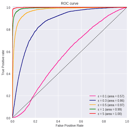
values=[predictions_dp, predictions_dp_1, predictions_dp_2, predictions_dp_3, predictions_dp_4]
titles=['ε = 0.1', 'ε = 0.3', 'ε = 0.5', 'ε = 1', 'ε = 5']
colors=['deeppink', 'navy', 'orange', 'green', 'red']
linestyle=['-','-','-','-','-']

plot_all_roc_curves(test_labels, values, titles, colors, linestyle)

We can see the impact of using different ε, we need to choose an example for comparison. The decision should take into consideration how much privacy we need and how much can the model tolerate noise until the performance starts declining.

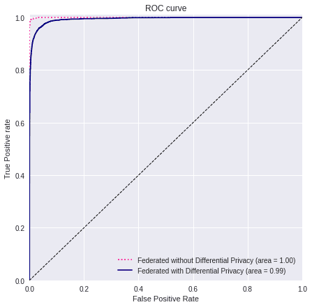
In this case, we will chose the 4th experiment where the ε values is 1, and see how much of a difference it makes compared to the model without Differential Privacy.

values=[predictions, predictions_dp_3]
titles=['Federated without Differential Privacy', 'Federated with Differential Privacy']
colors=['deeppink', 'navy']
linestyle=[':','-']

plot_all_roc_curves(test_labels, values, titles, colors, linestyle)

If we compare the 2 models, we can see that with this privacy configuration the performance is slightly worse. Nevertheless, it is still high, plus now we have Differential Privacy implemented on the weights of the model, adding an extra layer of security that will not reveal sensitive information.

However, only calculating a metric could make the evaluation a little bit biased, so it is recommendable to use another comparison value just to be sure. This way, we will now measure the F1-score.

5.2) F1 score

Another metric used is the F1 score, which seeks the balance between precision and recall values. This metric will allow us to estimate performance in another way and see the impact of Differential Privacy on it.

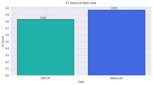
Calculating it, we can see that the results are much similar to that of the ROC AUC, confirming that a decent privacy budget still mantains the model perfectly usable.

values_f1 = predictions.argmax(axis=-1)
values_f1= np.eye(n_classes)[values_f1]

values_dp_3_f1 = predictions_dp_3.argmax(axis=-1)
values_dp_3_f1 = np.eye(n_classes)[values_dp_3_f1]

score_fed=f1_score(test_labels, values_f1, average='macro')
score_dp=f1_score(test_labels, values_dp_3_f1, average='macro')

values=[round(score_dp, 3),
        round(score_fed, 3)]

titles=['With DP',
        'Without DP']

colors=['lightseagreen',
        'royalblue']

plot_all_metric(values, "F1-Score" ,titles, colors)

With this last graph we can observe two results:

• F1 score is a metric that help us to understand the performance of our model. The ROC-AUC of these two experiments, gave us a really similar metric. On contrast, this last graph of the F1-Score demonstrate that they have different behaviours.

• Differential Privacy deteriorates the F1 metric. Even though it is a reduction of 0.111, it is a privacy layer that has been added, so the data of the individual is even more protected. For this reason, one has to find the trade-off of privacy versus utility of the model. If we add so much differential privacy, the data will be protected in the sense that it will be impossible to be recovered. But if we do that, the model utility is lost.

With this notebook, we have demonstrated that different values of the privacy budget $ε$, changes the utility of the model by adding more or less privacy. $ε$, then, is not fixed and will depend on the concrete problem and the amount of privacy that we want to apply to it.