Federated models: linear regression

Here, we explain how to set up a Linear Regression experiment in the Federated setting using the Sherpa.ai Federated Learning and Differential Privacy Framework. Results from federated learning are compared to (non-federated) centralized learning. Moreover, we also show how the addition of differential privacy affects the performance of the federated model. Ultimately, an application of the composition theorems for adaptive differential privacy is given.

Index

1) The data

In the present example, we will use the California Housing dataset from sklearn. We only make use of two features, in order to reduce the variance in the prediction. The Sherpa.ai Federated Learning and Differential Privacy Framework allows a generic dataset to easily be converted, to interact with the platform:

import shfl
from shfl.data_base.data_base import WrapLabeledDatabase
import sklearn.datasets
import numpy as np
from shfl.auxiliar_functions_for_notebooks.functionsFL import *
from shfl.private.reproducibility import Reproducibility
import matplotlib.pyplot as plt

Reproducibility(1234)

all_data = sklearn.datasets.fetch_california_housing()
n_features = 2
data = all_data["data"][:,0:n_features]
labels = all_data["target"]    

# Retain part for DP sensitivity sampling:
size = 2000
sampling_data = data[-size:, ]
sampling_labels = labels[-size:, ]

# Create database:
database = WrapLabeledDatabase(data[0:-size, ], labels[0:-size])
train_data, train_labels, test_data, test_labels = database.load_data()

2022-03-24 18:09:28.534469: W tensorflow/stream_executor/platform/default/dso_loader.cc:64] Could not load dynamic library 'libcudart.so.11.0'; dlerror: libcudart.so.11.0: cannot open shared object file: No such file or directory
2022-03-24 18:09:28.534485: I tensorflow/stream_executor/cuda/cudart_stub.cc:29] Ignore above cudart dlerror if you do not have a GPU set up on your machine.

print("Shape of training and test data: " + str(train_data.shape) + str(test_data.shape))
print("Total: " + str(train_data.shape[0] + test_data.shape[0]))

Shape of training and test data: (14912, 2)(3728, 2)
Total: 18640

We will simulate a FL scenario by distributing the training data over a collection of clients, assuming an IID setting:

iid_distribution = shfl.data_distribution.IidDataDistribution(database)
nodes_federation, test_data, test_labels = iid_distribution.get_nodes_federation(num_nodes=5)

from shfl.model.linear_regression_model import LinearRegressionModel

def model_builder():
    model = LinearRegressionModel(n_features=n_features, n_targets=1)
    return model

aggregator = shfl.federated_aggregator.FedAvgAggregator()

3) Run the federated learning experiment

We're now ready to run the FL model. The Sherpa.ai Federated Learning and Differential Privacy Framework offers support for the Linear Regression model from scikit-learn. The user must specify the number of features and targets, in advance. Note that in this case, we set the number of rounds to 1 since no iterations are needed in the case of linear regression. The performance metrics used are the Root Mean Squared Error (RMSE) and the $R^2$ score. It can be observed that the performance of the global model (i.e., the aggregated model) is generally superior with respect to the performance of each node, thus, the federated learning approach proves to be beneficial:

federated_government = shfl.federated_government.FederatedGovernment(model_builder(), nodes_federation, aggregator)
federated_government.run_rounds(n_rounds=1, test_data=test_data, test_label=test_labels)

Evaluation in round 0:

Collaborative model test -> RMSE: 0.8259307991985892  r2_score: 0.49386103506084966  

And we can observe that the performance is comparable to the centralized learning model:

# Comparison with centralized model:
centralized_model = LinearRegressionModel(n_features=n_features, n_targets=1)
centralized_model.train(data=train_data, labels=train_labels)
print(centralized_model.evaluate(data=test_data, labels=test_labels))

[('RMSE', 0.825926355176148), ('r2_score', 0.49386648173233705)]

4) Add differential privacy

We want to assess the impact of differential privacy (see The Algorithmic Foundations of Differential Privacy, Section 3.3) on the federated model's performance.

4.1) Model's sensitivity

In the case of applying the Laplace privacy mechanism, the noise added has to be of the same order as the sensitivity of the model's output, i.e., the model parameters of our linear regression. In the general case, the model's sensitivity might be difficult to compute analytically. An alternative approach is to attain random differential privacy through a sampling over the data (e.g., see Rubinstein 2017. That is, instead of computing the global sensitivity $\Delta f$ analytically, we compute an empirical estimation of it by sampling over the dataset. However, be advised that this will guarantee the weaker property of random differential privacy. This approach is convenient, since it allows for the sensitivity estimation of an arbitrary model or a black-box computer function. The Sherpa.ai Federated Learning and Differential Privacy Framework provides this functionality in the class SensitivitySampler.

We need to specify a distribution of the data to sample from. Generally, this requires previous knowledge and/or model assumptions. In order not to make any specific assumptions about the distribution of the dataset, we can choose a uniform distribution. We define our class of ProbabilityDistribution that uniformly samples over a data-frame. We use the previously retained part of the dataset for sampling:

class UniformDistribution(shfl.differential_privacy.ProbabilityDistribution):
    """
    Implement Uniform sampling over the data
    """
    def __init__(self, sample_data):
        self._sample_data = sample_data

    def sample(self, sample_size):
        row_indices = np.random.randint(low=0, high=self._sample_data.shape[0], size=sample_size, dtype='l')
        
        return self._sample_data[row_indices, :]
    
sample_data = np.hstack((sampling_data, sampling_labels.reshape(-1,1)))

The class SensitivitySampler implements the sampling, given a query, i.e., the learning model itself, in this case. We only need to add the get method to our model since it is required by the class SensitivitySampler. We choose the sensitivity norm to be the $L_1$ norm and we apply the sampling. Typically, the value of the sensitivity is influenced by the size of the sampled data: the higher, the more accurate the sensitivity.

from shfl.differential_privacy.sensitivity_sampler import SensitivitySampler
from shfl.differential_privacy.norm import L1SensitivityNorm

class LinearRegressionSample(LinearRegressionModel):
    
    def __call__(self, data_array):
        data = data_array[:, 0:-1]
        labels = data_array[:, -1]
        train_model = self.train(data, labels)
      
        return self.get_model_params()

distribution = UniformDistribution(sample_data)
sampler = SensitivitySampler()
n_data_size = 4000
max_sensitivity, mean_sensitivity = sampler.sample_sensitivity(
    LinearRegressionSample(n_features=n_features, n_targets=1), 
    L1SensitivityNorm(), distribution, n_data_size=n_data_size, gamma=0.05)
print("Max sensitivity from sampling: " + str(max_sensitivity))
print("Mean sensitivity from sampling: " + str(mean_sensitivity))

Max sensitivity from sampling: [0.015044483412654852, 0.0030757411817898465]
Mean sensitivity from sampling: [0.0005688578783578508, 0.00011888312830760566]

Unfortunately, sampling over a dataset involves the training of the model on two datasets differing in one entry, at each sample. Thus, in general, this procedure might be computationally expensive (e.g. in the case of training a deep neural network).

4.2) Run the federated learning experiment with differential privacy

At this stage, we are ready to add a layer of DP to our federated learning model. We will apply the Laplace mechanism, employing the sensitivity obtained from the previous sampling. The Laplace mechanism provided by the Sherpa.ai Federated Learning and Differential Privacy Framework is then assigned as the private access type to the model parameters of each client in a new FederatedGovernment object. This results in an $\epsilon$-differentially private FL model. For example, by choosing the value $\epsilon = 0.5$, we can run the FL experiment with DP:

from shfl.differential_privacy.mechanism import LaplaceMechanism

params_access_definition = LaplaceMechanism(sensitivity=max_sensitivity, epsilon=0.5)
nodes_federation.configure_model_params_access(params_access_definition);

federated_governmentDP = shfl.federated_government.FederatedGovernment(
    model_builder(), nodes_federation, aggregator)
federated_governmentDP.run_rounds(n_rounds=1, test_data=test_data, test_label=test_labels)

Evaluation in round 0:

Collaborative model test -> RMSE: 0.8284132227702525  r2_score: 0.4908139529133695  

In the above example we saw that the performance of the model deteriorated slightly, due to the addition of differential privacy. It must be noted that each run involves a different random noise added by the differential privacy mechanism. However, in general, privacy increases at the expense of accuracy (i.e. for smaller values of $\epsilon$). This can be observed by calculating a mean of several runs, as explained below.

4.3) Comparing the metrics

Now that we have all the models, let's do the metrics calculations:

from shfl.auxiliar_functions_for_notebooks.functionsFL import *
import matplotlib.pyplot as plt

fed_model = federated_government._server._model
evaluation_fed = fed_model.evaluate(train_data, train_labels)


dp_model = federated_governmentDP._server._model
evaluation_dp = dp_model.evaluate(train_data, train_labels)

evaluation_cent = centralized_model.evaluate(data=test_data, labels=test_labels)

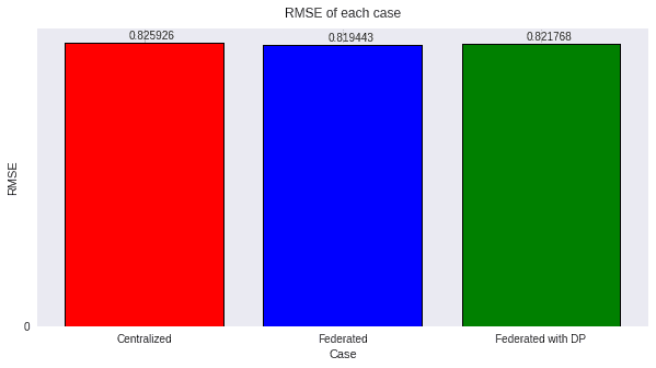
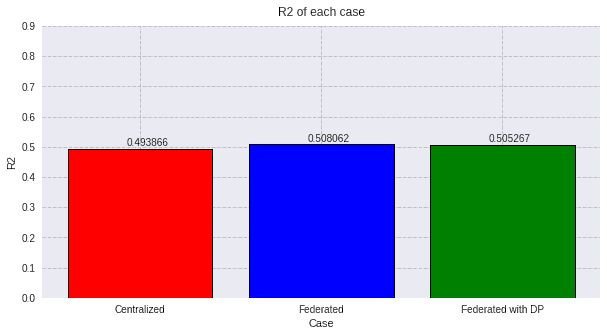
We are evaluating the Root Mean Squared Error and the R2 coefficient, and then, the R2 coefficient, and plotting the values from all the models:

values=[round(evaluation_cent[0][1], 6), round(evaluation_fed[0][1], 6), round(evaluation_dp[0][1], 6)]
titles=['Centralized', 'Federated', 'Federated with DP']
colors=['red', 'blue', 'green']
plot_all_RMSE(values, titles, colors, 1)

values=[round(evaluation_cent[1][1], 6), round(evaluation_fed[1][1], 6), round(evaluation_dp[1][1], 6)]
plot_all_R2(values, titles, colors)

As expected, the federated case behaves much alike the centralized model, but when adding a high privacy $\epsilon$ coefficient the performance is slightly hindered.