⚠

Please note that these tutorials refer to a deprecated version of the platform. The current version of the platform, which is not publicly available, has a more advanced architecture and provides a wider range of functionalities. These tutorials are only for illustrative purposes and showcase a limited number of the platform’s capabilities.

Federated models: K-means clustering

This notebook covers the problem of unsupervised learning in a federated configuration. In particular, a K-means clustering is used from the sklearn library (see this link). This model is encapsulated in the Sherpa.ai FL platform and it is thus ready to use.

Index

1) The data

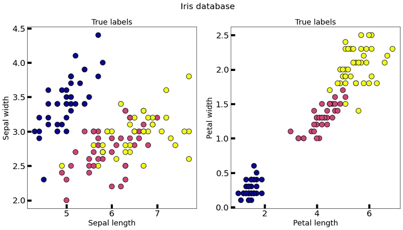
The framework provides a function to load the Iris dataset.

import matplotlib.pyplot as plt
import shfl
import numpy as np
from shfl.data_base.iris import Iris


# Assign database:
database = Iris()

train_data, train_labels, test_data, test_labels = database.load_data()

# Visualize training data: 
fig, ax = plt.subplots(1,2, figsize=(16,8))
fig.suptitle("Iris database", fontsize=20)
ax[0].set_title('True labels', fontsize=18)
ax[0].scatter(train_data[:, 0], train_data[:, 1], c=train_labels, s=150, edgecolor='k', cmap="plasma")
ax[0].set_xlabel('Sepal length', fontsize=18)
ax[0].set_ylabel('Sepal width', fontsize=18)
ax[0].tick_params(direction='in', length=10, width=5, colors='k', labelsize=20)

ax[1].set_title('True labels', fontsize=18)
ax[1].scatter(train_data[:, 2], train_data[:, 3], c=train_labels, s=150, edgecolor='k', cmap="plasma")
ax[1].set_xlabel('Petal length', fontsize=18)
ax[1].set_ylabel('Petal width', fontsize=18)
ax[1].tick_params(direction='in', length=10, width=5, colors='k', labelsize=20)

plt.show()

2022-03-24 17:40:52.768768: W tensorflow/stream_executor/platform/default/dso_loader.cc:64] Could not load dynamic library 'libcudart.so.11.0'; dlerror: libcudart.so.11.0: cannot open shared object file: No such file or directory
2022-03-24 17:40:52.768784: I tensorflow/stream_executor/cuda/cudart_stub.cc:29] Ignore above cudart dlerror if you do not have a GPU set up on your machine.

png

2) The model

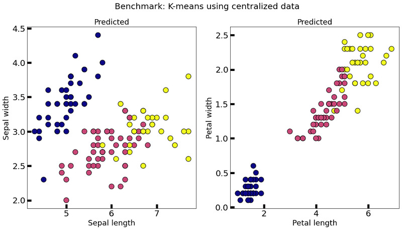
We implement a method to plot K-means results in the Iris database and establish a centralized model, which will be our reference model.

from shfl.model.kmeans_model import KMeansModel

def plot_k_means(km, X, title):
    new_labels=km.predict(X)
    fig, axes=plt.subplots(1, 2, figsize=(16,8))
    fig.suptitle(title, fontsize=20)
    axes[0].scatter(X[:, 0], X[:, 1], c=new_labels, cmap='plasma', edgecolor='k', s=150)
    axes[0].set_xlabel('Sepal length', fontsize=18)
    axes[0].set_ylabel('Sepal width', fontsize=18)
    axes[0].tick_params(direction='in', length=10, width=5, colors='k', labelsize=20)
    axes[0].set_title('Predicted', fontsize=18)
    
    axes[1].scatter(X[:, 2], X[:, 3], c=new_labels, cmap='plasma', edgecolor='k', s=150)
    axes[1].set_xlabel('Petal length', fontsize=18)
    axes[1].set_ylabel('Petal width', fontsize=18)
    axes[1].tick_params(direction='in', length=10, width=5, colors='k', labelsize=20) 
    axes[1].set_title('Predicted', fontsize=18)
    
# Plot training data:
centralized_model = KMeansModel(n_clusters=3, n_features=train_data.shape[1])
centralized_model.train(train_data)

plot_k_means(centralized_model, train_data, title="Benchmark: K-means using centralized data")

png

2.1) How to _aggregate a model's parameters from each federated node in clustering

Since the labels of clusters can vary among each node, we cannot average the centroids right away. One solution is to choose the lowest distance average: this is achieved by simply applying the K-means algorithm to the centroids coordinates of all nodes.

Note: This implementation is based on the assumption that the number of clusters has been previously fixed across the clients, so it only works properly in IID scenarios.

from shfl.federated_aggregator.cluster_fedavg_aggregator import cluster_fed_avg_aggregator

# Create the IID data: 
iid_distribution = shfl.data_distribution.IidDataDistribution(database)
nodes_federation, test_data, test_label = iid_distribution.get_nodes_federation(num_nodes=12, percent=100)

# Run the algorithm:
aggregator = cluster_fed_avg_aggregator

3) Run the federated learning experiment

We are now ready to run our model in a federated configuration.

The performance is assessed by several clustering metrics (see this link).

For reference, below, we compare the metrics of:

Each node
The global (federated) model
The centralized (non-federated) model

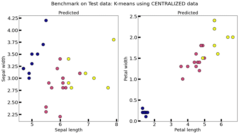
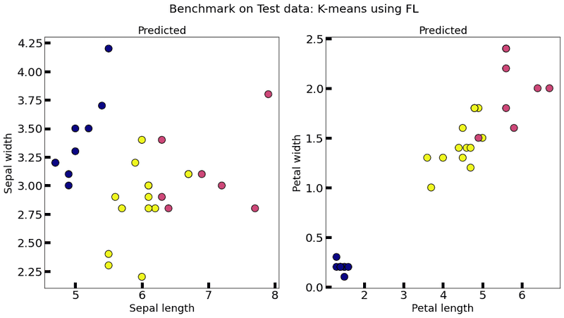
It can be observed that the performance of the global federated model is superior, in general, with respect to the performance of each node. Thus, the federated learning approach proves to be beneficial. Moreover, the performance of the global federated model is very close to the performance of the centralized model.

from shfl.federated_government.federated_government import FederatedGovernment

n_clusters = 3 # Set number of clusters
n_features = train_data.shape[1]
def model_builder():
    model=KMeansModel(n_clusters=n_clusters, n_features=n_features)
    return model


federated_government=FederatedGovernment(model_builder(), nodes_federation, aggregator)
print("Test data size: " + str(test_data.shape[0]))
print("\n")
federated_government.run_rounds(n_rounds=3, test_data=test_data, test_label=test_label)

# Reference centralized (non federate) model:
print("Centralized model test performance : ", end='')

for metric in centralized_model.evaluate(data=test_data, labels=test_labels):
    print(metric[0]+": "+str(metric[1]), end='  ')

plot_k_means(centralized_model, test_data, title="Benchmark on Test data: K-means using CENTRALIZED data")
plot_k_means(federated_government._server._model, test_data, title="Benchmark on Test data: K-means using FL")

Test data size: 30


Evaluation in round 0:

Collaborative model test -> homogeneity_score: 0.6945415531906901  completeness_score: 0.7069597474605258  v_measure_score: 0.7006956337698431  adjusted_rand_score: 0.6406094330911477  

Evaluation in round 1:

Collaborative model test -> homogeneity_score: 0.6945415531906901  completeness_score: 0.7069597474605258  v_measure_score: 0.7006956337698431  adjusted_rand_score: 0.6406094330911477  

Evaluation in round 2:

Collaborative model test -> homogeneity_score: 0.6945415531906901  completeness_score: 0.7069597474605258  v_measure_score: 0.7006956337698431  adjusted_rand_score: 0.6406094330911477  

Centralized model test performance : homogeneity_score: 0.69454155319069  completeness_score: 0.7069597474605257  v_measure_score: 0.7006956337698431  adjusted_rand_score: 0.6406094330911477

png

4) Add differential privacy

To preserve client privacy, in this section, we are going to introduce Differential Privacy (DP) into our model. First, we calibrate the noise introduced by the differentially private mechanism using the training data, then we apply DP to each client feature, so that each cluster computed by a client is shared with the main server privately; that is, without disclosing the identity of the client.

4.1) Model's sensitivity

In the case of applying the Gaussian privacy mechanism, the noise added has to be of the same order as the sensitivity of the model's output, i.e., the coordinates of each cluster.

In the general case, the model's sensitivity might be difficult to compute analytically. An alternative approach is to attain random differential privacy through a sampling over the data.

That is, instead of computing the global sensitivity $\Delta f$ analytically, we compute an empirical estimation of it, by sampling over the dataset. This approach is very convenient, since it allows for the sensitivity estimation of an arbitrary model or a black-box computer function.

In order to carry out this approach, we need to specify a distribution of the data to sample from. Generally, this requires previous knowledge and/or model assumptions. However, in our specific case of manufactured data, we can assume that the data distribution is uniform. We define our class of ProbabilityDistribution that uniformly samples over a data-frame. Moreover, we assume that we have access to a set of data (this can be thought of, for example, as a public data set). In this example, we generate a new dataset, and use its training partition for sampling:

import numpy as np

class UniformDistribution(shfl.differential_privacy.ProbabilityDistribution):
    """
    Implement Uniform sampling over the data
    """
    def __init__(self, sample_data):
        self._sample_data=sample_data

    def sample(self, sample_size):
        row_indices=np.random.randint(low=0, high=self._sample_data.shape[0], size=sample_size, dtype='l')
        
        return self._sample_data[row_indices, :]
    
sample_data = train_data

The class SensitivitySampler implements the sampling, given a query, i.e., the learning model itself, in this case. We only need to add the __call__ method to our model since it is required by the class SensitivitySampler to make the query callable. We choose the sensitivity norm to be the v norm and we apply the sampling. Typically, the value of the sensitivity is influenced by the size of the sampled data: the higher, the more accurate the sensitivity.

Unfortunately, sampling over a dataset involves the training of the model on two datasets differing in one entry, at each sample. Thus, in general, this procedure might be computationally expensive (e.g., in the case of training a deep neural network).

from shfl.differential_privacy import SensitivitySampler
from shfl.differential_privacy import L2SensitivityNorm

class KMeansSample(KMeansModel):
    
    def __init__(self, feature, **kargs):
        self._feature=feature
        super().__init__(**kargs)
    
    def __call__(self, data_array):
        self.train(data_array)
        params=self.get_model_params()
        return params[:, self._feature]

distribution = UniformDistribution(sample_data)
sampler = SensitivitySampler()
# Reproducibility
np.random.seed(789)
n_data_size=50

sensitivities = np.empty(n_features)

for i in range(n_features):
    model=KMeansSample(feature=i, n_clusters=n_clusters, n_features=n_features)
    sensitivities[i], _=sampler.sample_sensitivity(model, 
                                                   L2SensitivityNorm(), 
                                                   distribution, 
                                                   n_data_size=n_data_size, 
                                                   gamma=0.05)
    
    print("Done feature: {}/{}.\n".format((i+1), n_features))

Done feature: 1/4.

Done feature: 2/4.

Done feature: 3/4.

Done feature: 4/4.

print("Max sensitivity from sampling: ", np.max(sensitivities))
print("Min sensitivity from sampling: ", np.min(sensitivities))
print("Mean sensitivity from sampling:", np.mean(sensitivities))

Max sensitivity from sampling:  6.788248117150698
Min sensitivity from sampling:  1.5088413367199793
Mean sensitivity from sampling: 3.6169284933281967

Generally, if the model has more than one feature, it is a bad idea to estimate the sensitivity for all of the features at the same time, as the features may have wildly varying sensitivities. In this case, we estimate the sensitivity for each feature. Note that we provide the array of estimated sensitivities to the GaussianMechanism and apply it to each feature individually.

4.2) Run the federated learning experiment with differential privacy

At this stage we are ready to add the layer of DP to our federated learning model:

from shfl.differential_privacy import GaussianMechanism

dpm = GaussianMechanism(sensitivity=sensitivities, epsilon_delta=(0.9, 0.9))
nodes_federation.configure_model_params_access(dpm)

federated_government = FederatedGovernment(model_builder(), nodes_federation, aggregator)

federated_government.run_rounds(n_rounds=1, test_data=test_data, test_label=test_label)

# Reference centralized (non federate) model:
print("Centralized model test performance : ", end='')

for metric in centralized_model.evaluate(data=test_data, labels=test_labels):
    print(metric[0]+": "+str(metric[1]), end='  ')
    
plot_k_means(centralized_model, test_data, title="Benchmark on Test data: K-means using CENTRALIZED data")
plot_k_means(federated_government._server._model, test_data, title="Benchmark on Test data: K-means using FL and DP")

Evaluation in round 0:

Collaborative model test -> homogeneity_score: 0.7786209392201336  completeness_score: 0.8072541028593236  v_measure_score: 0.7926790334419561  adjusted_rand_score: 0.71795302819269  

Centralized model test performance : homogeneity_score: 0.69454155319069  completeness_score: 0.7069597474605257  v_measure_score: 0.7006956337698431  adjusted_rand_score: 0.6406094330911477

png

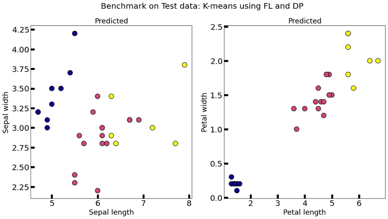
As you can see, when we add DP to the model, it becomes quite unstable (multiple executions each one with very different results) and almost useless (even with unacceptable values for $\delta$ , that is $\delta \geq 0.5$ , the results are quite bad), which suggests that another way of adding DP has to be provided. An alternative approach for adding DP can be found in A differential privacy protecting K-means clustering algorithm based on contour coefficients, but it is still unclear as to how to adapt it to a federated setting.