Federated learning: deep learning for vertically partitioned data
In this notebook, we provide a simple example of how to perform a vertical federated learning experiment with the help of the Sherpa.ai Federated Learning framework. As opposed to the horizontal federated learning paradigm, in a vertical federated learning setting (see e.g. Federated Machine Learning: Concept and Applications) the different nodes possess the same samples, but different features. A practical example being that of a local on-line shop and an insurance company: both entities might have matching customers (samples), but the information (features) each entity possesses about the customers is of different nature. We are going to use a synthetic dataset and a neural network model.
The data
We use sklearn module for generating synthetic databases.
Moreover, in order to simulate a vertically partitioned training data, we randomly split the features of the created dataset among the clients:
import numpy as np
import pandas as pd
import matplotlib.pyplot as plt

from sklearn import preprocessing
from sklearn.metrics import roc_curve, auc
from sklearn.linear_model import LogisticRegression
from sklearn.neural_network import MLPClassifier
from sklearn.datasets import make_classification
from shfl.private.reproducibility import Reproducibility

# Comment to turn off reproducibility:
Reproducibility(567)

# Create dataset
n_features = 20
n_classes = 2
n_samples = 15000

data, labels = make_classification(
    n_samples=n_samples, n_features=n_features,
    n_redundant=0, n_repeated=0, n_classes=n_classes,
    n_clusters_per_class=1, flip_y=0.1, class_sep=0.4, random_state=123)
2022-03-23 10:42:30.935246: W tensorflow/stream_executor/platform/default/dso_loader.cc:64] Could not load dynamic library 'libcudart.so.11.0'; dlerror: libcudart.so.11.0: cannot open shared object file: No such file or directory
2022-03-23 10:42:30.935264: I tensorflow/stream_executor/cuda/cudart_stub.cc:29] Ignore above cudart dlerror if you do not have a GPU set up on your machine.
/home/f.palomino/Desktop/venvpruebas/environment/lib/python3.8/site-packages/tqdm/auto.py:22: TqdmWarning: IProgress not found. Please update jupyter and ipywidgets. See https://ipywidgets.readthedocs.io/en/stable/user_install.html
from .autonotebook import tqdm as notebook_tqdmVertical split of the dataset. In the vertical FL setting, the database is split along the columns (i.e., vertically) among the nodes. We can use a method provided by the Sherpa FL Framework to randomly split a dataset vertically into the desired number of parts:
from shfl.data_base.data_base import vertical_split

# Create a vertically split dataset: split the features among clients
M = 2  # number of clients
train_data, train_labels, test_data, test_labels = \
    vertical_split(data=data, labels=labels)

for item in train_data:
    print("Client train data shape: " + str(item.shape))
Client train data shape: (12000, 10)
Client train data shape: (12000, 10)Wrap into NodesFederation. At this point, we assign the data to a federated network of clients.
Since the clients actually don't possess the labels (only the server does), we assign the client's labels to None.
And since we already performed the split of data for each client, we just need convert it to federated data:
# Convert to federated data:
from shfl.private.federated_operation import federate_list

nodes_federation = federate_list(train_data)
print(nodes_federation)
<shfl.private.federated_operation.NodesFederation object at 0x7fcbf0d08fa0>In order to visually check everything went fine with the data assignment, we can configure data access to node (otherwise protected by default):
# Check federated data:
from shfl.private.utils import unprotected_query

nodes_federation.configure_data_access(unprotected_query);
nodes_federation[0].query()
nodes_federation[0].query().data.shape
#nodes_federation[0].query().label
print(nodes_federation[0].query().data.dtype)float64The model:
Horizontal Vs Vertical Federated Learning. Both in the Federated Government is interpreted as follows:
- The Federated Government is intended as a Coordinator: it defines and schedules the federated computations, but does not have any other function (no data, no model). It is what a user can customize for the specific case problem.
- The Federated Data is composed by nodes that can have multiple functions: train, store data, _aggregate, make auxiliary computations, predictions etc.
- In particular, the Server is itself a node that can interact with the Federated Data: it might _aggregate, but might also contain data and train on them
In Horizontal FL (see e.g. the basic concepts notebook), all nodes have typically the same model, and the server node has also the aggregation function in its model as an attribute but do not train and does not possess any data. Instead in a Vertical FL architecture, the client nodes might have a different model with respect each other and with respect the server node. The latter in turn can _aggregate, train and might possess its own data (i.e. the labels in this case).
Note that the distinction between client and server is only virtual and not necessarily physical, since a single node might be both client and server, allowing multiple roles for the same physical node.
Define the server node. We said that in the Vertical FL, each node, including the server, is allowed to possess a different model and different methods for interacting with the clients. We here define the server model with specific functions needed for the present Vertical FL architecture. The server is assigned a linear model, along with the data to train on (only labels, in this specific example):
import torch
import torch.nn as nn
from sklearn.metrics import roc_auc_score

from shfl.model.vertical_deep_learning_model import VerticalNeuralNetServerModel
from shfl.private.federated_operation import VerticalServerDataNode
from shfl.private.data import LabeledData

n_embeddings = 2

model_server = torch.nn.Sequential(
    torch.nn.Linear(n_embeddings, 1, bias=True),
    torch.nn.Sigmoid())

loss_server = torch.nn.BCELoss(reduction="mean")
optimizer_server = torch.optim.SGD(params=model_server.parameters(), lr=0.001)


def roc_auc(y_pred, y_true):
    """
    # Arguments:
        y_pred: Predictions
        y_true: True labels
    """
    return roc_auc_score(y_true, y_pred)

model = VerticalNeuralNetServerModel(model_server, loss_server, optimizer_server,
                                      metrics={"roc_auc": roc_auc})
from shfl.federated_aggregator import FedSumAggregator
# Create the server node:
server_node = VerticalServerDataNode(
nodes_federation=nodes_federation,
model=model,
aggregator=FedSumAggregator(),
data=LabeledData(data=None, label=train_labels.reshape(-1,1).astype(np.float32)))for layer in model_server.parameters():
print(layer)Parameter containing:
tensor([[-0.6730, 0.2561]], requires_grad=True)
Parameter containing:
tensor([0.6738], requires_grad=True)Define specific data access needed for the Vertical FL round. The specific Vertical FL architecture requires the computation of the Loss and the exchange of convergence parameters. Namely, the clients send the computed embeddings to the server, and the server sends the computed gradients to update the clients. Therefore, we define ad-hoc access definitions for these methods, and we assign them to server and clients:
def train_set_evaluation(data, **kwargs):
    """Evaluate collaborative model on batch train data."""
    server_model = kwargs.get("server_model")
    embeddings, embeddings_indices = kwargs.get("meta_params")
    labels = data.label[embeddings_indices]

    evaluation = server_model.evaluate(embeddings, labels)

    return evaluation


def meta_params_query(model, **kwargs):
    """Returns embeddings (or their gradients) as computed by the local model."""
    return model.get_meta_params(**kwargs)


# Configure data access to nodes and server
nodes_federation.configure_model_access(meta_params_query)
server_node.configure_model_access(meta_params_query)
server_node.configure_data_access(train_set_evaluation)

print(nodes_federation[1]._model_access_policy)
print(server_node._model_access_policy)
print(server_node._private_data_access_policies)
<function meta_params_query at 0x7fcbeeccb9d0>
<function meta_params_query at 0x7fcbeeccb9d0>
{'140513895288736': <function train_set_evaluation at 0x7fcbeeccb8b0>}Run the federated learning experiment
We are almost done: we only need to specify which specific model to use for each client node, and the server node.
Namely, the clients will run a neural network model, but of course they will have different input size since they possess different number of features.
We first don't use hidden layers for the clients model, resulting in a linear model (layer_dims=None parameter):
from shfl.model.vertical_deep_learning_model import VerticalNeuralNetClientModel

model0 = nn.Sequential(
    nn.Linear(train_data[0].shape[1], n_embeddings, bias=True),
)

model1 = nn.Sequential(
    nn.Linear(train_data[1].shape[1], n_embeddings, bias=True),
)

optimizer0 = torch.optim.SGD(params=model0.parameters(), lr=0.001)
optimizer1 = torch.optim.SGD(params=model1.parameters(), lr=0.001)

batch_size = 32
model_nodes = [VerticalNeuralNetClientModel(model=model0, loss=None, optimizer=optimizer0, batch_size=batch_size),
               VerticalNeuralNetClientModel(model=model1, loss=None, optimizer=optimizer1, batch_size=batch_size)]
for layer in model0.parameters():
print(layer)
for layer in model1.parameters():
print(layer)
Parameter containing:
tensor([[-0.3068,  0.2944, -0.2563, -0.3143, -0.2763, -0.0413,  0.2372, -0.1069,
            -0.2783, -0.1169],
        [ 0.0033,  0.0914, -0.1566, -0.0794, -0.0943, -0.0910,  0.2255,  0.2800,
            -0.2242, -0.1920]], requires_grad=True)
Parameter containing:
tensor([ 0.0059, -0.2826], requires_grad=True)
Parameter containing:
tensor([[-0.1106, -0.3151,  0.0279, -0.2343, -0.3058, -0.1020, -0.2026, -0.1507,
            -0.1658, -0.0334],
        [-0.2455,  0.2706, -0.2163, -0.1849, -0.1603,  0.2718,  0.3025, -0.2665,
            0.0953,  0.3116]], requires_grad=True)
Parameter containing:
tensor([0.0902, 0.0599], requires_grad=True)
Pytorch models expect by default input data to be float, and if they are in double precision it raises an error.
We have two options: either convert the node models just created from the default float to double, or convert the input data to float.
If we are not concerned about having double precision, but rather we prefer faster computation, we opt for the second strategy. We apply a federated transformation:
def cast_to_float(labeled_data):
    if labeled_data.data is not None:
        labeled_data.data = labeled_data.data.astype(np.float32)

nodes_federation.apply_data_transformation(cast_to_float);
from shfl.federated_government.vertical_federated_government import VerticalFederatedGovernment
# Create federated government:
federated_government = VerticalFederatedGovernment(model_nodes,
nodes_federation,
server_node=server_node)# Run training:
federated_government.run_rounds(n_rounds=10001,
test_data=test_data,
test_label=test_labels.reshape(-1,1),
eval_freq=1000)Evaluation in round 0 :
Loss: 0.7352080345153809 Accuracy: 0.5861049966663983
Evaluation in round 1000 :
Loss: 0.6777400970458984 Accuracy: 0.6498390575358746
Evaluation in round 2000 :
Loss: 0.636843204498291 Accuracy: 0.7063939770112693
Evaluation in round 3000 :
Loss: 0.6027745604515076 Accuracy: 0.7540046585915966
Evaluation in round 4000 :
Loss: 0.5727333426475525 Accuracy: 0.7916425560607725
Evaluation in round 5000 :
Loss: 0.5458422303199768 Accuracy: 0.8191826871542695
Evaluation in round 6000 :
Loss: 0.5225133299827576 Accuracy: 0.8373633812639577
Evaluation in round 7000 :
Loss: 0.5032355189323425 Accuracy: 0.8490681260088092
Evaluation in round 8000 :
Loss: 0.4881543815135956 Accuracy: 0.8558296220420678
Evaluation in round 9000 :
Loss: 0.4768766164779663 Accuracy: 0.8593860568718228
Evaluation in round 10000 :
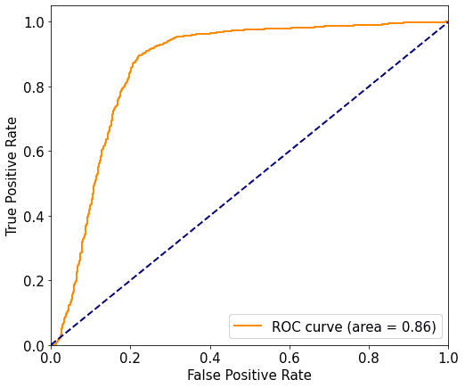
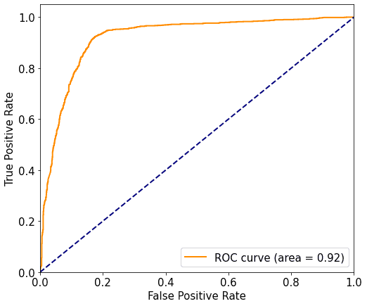
Loss: 0.4686449468135834 Accuracy: 0.8613235043603688Comparison to Centralized training. As reference, we can compare the performance of the collaborative model to the centralized training:
def plot_roc(y_test, y_prediction, save_path=None):
    fpr, tpr, _ = roc_curve(y_test, y_prediction)
    roc_auc = auc(fpr, tpr)
    plt.rcParams.update({'font.size': 15})
    plt.figure(figsize=(8, 7))
    lw = 2
    plt.plot(fpr, tpr, color='darkorange',
             lw=lw, label='ROC curve (area = %0.2f)' % roc_auc)
    plt.plot([0, 1], [0, 1], color='navy', lw=lw, linestyle='--')
    plt.xlim([0.0, 1.0])
    plt.ylim([0.0, 1.05])
    plt.xlabel('False Positive Rate')
    plt.ylabel('True Positive Rate')
    plt.legend(loc="lower right")
    if save_path is not None:
        plt.savefig(save_path, bbox_inches = "tight")
    plt.show()
y_prediction = federated_government._server.predict_collaborative_model(test_data)
plot_roc(test_labels, y_prediction)

# Linear model Benchmark on centralized data using sk-learn:
centralized_train_data = np.concatenate(train_data, axis=1)
centralized_test_data = np.concatenate(test_data, axis=1)
clf_linear = LogisticRegression(random_state=123).fit(centralized_train_data, train_labels)
y_prediction = clf_linear.predict_proba(centralized_test_data)[:, 1]
plot_roc(test_labels, y_prediction)

Non-linear model:
We now add a hidden layer in the clients' neural network model, resulting in a non-linear model. Namely, we will use a hidden layer in the clients' models:
n_hidden_neurons = 3
model0 = nn.Sequential(
nn.Linear(train_data[0].shape[1], n_hidden_neurons, bias=True),
nn.ReLU(),
nn.Linear(n_hidden_neurons, n_embeddings, bias=True)
)
model1 = nn.Sequential(
nn.Linear(train_data[1].shape[1], n_hidden_neurons, bias=True),
nn.ReLU(),
nn.Linear(n_hidden_neurons, n_embeddings, bias=True)
)
optimizer0 = torch.optim.SGD(params=model0.parameters(), lr=0.001)
optimizer1 = torch.optim.SGD(params=model1.parameters(), lr=0.001)
batch_size = 32
model_nodes = [VerticalNeuralNetClientModel(model=model0, loss=None, optimizer=optimizer0, batch_size=batch_size),
VerticalNeuralNetClientModel(model=model1, loss=None, optimizer=optimizer1, batch_size=batch_size)]from shfl.federated_government.vertical_federated_government import VerticalFederatedGovernment
# Create federated government and run training:
federated_government = VerticalFederatedGovernment(model_nodes,
nodes_federation,
server_node=server_node)federated_government.run_rounds(n_rounds=150001,
test_data=test_data,
test_label=test_labels.reshape(-1,1),
eval_freq=10000)Evaluation in round 0 :
Loss: 0.7225618362426758 Accuracy: 0.5035157377578537
Evaluation in round 10000 :
Loss: 0.4516731798648834 Accuracy: 0.8614862926479738
Evaluation in round 20000 :
Loss: 0.43100520968437195 Accuracy: 0.8646720060631966
Evaluation in round 30000 :
Loss: 0.4286576211452484 Accuracy: 0.8652408755163301
Evaluation in round 40000 :
Loss: 0.4275318682193756 Accuracy: 0.8654412474386419
Evaluation in round 50000 :
Loss: 0.4266299605369568 Accuracy: 0.8657316866512269
Evaluation in round 60000 :
Loss: 0.4259287118911743 Accuracy: 0.8661257588447191
Evaluation in round 70000 :
Loss: 0.42526376247406006 Accuracy: 0.8669312495246448
Evaluation in round 80000 :
Loss: 0.423758327960968 Accuracy: 0.8690521674193031
Evaluation in round 90000 :
Loss: 0.41741418838500977 Accuracy: 0.8760042502865474
Evaluation in round 100000 :
Loss: 0.4010367691516876 Accuracy: 0.8924907897856131
Evaluation in round 110000 :
Loss: 0.38908955454826355 Accuracy: 0.9003984754832388
Evaluation in round 120000 :
Loss: 0.37973856925964355 Accuracy: 0.906970496624367
Evaluation in round 130000 :
Loss: 0.37336766719818115 Accuracy: 0.9106955018393742
Evaluation in round 140000 :
Loss: 0.3677959740161896 Accuracy: 0.9149553510867452
Evaluation in round 150000 :
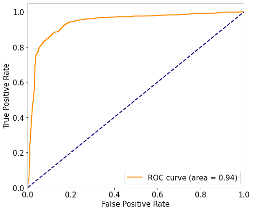
Loss: 0.36224597692489624 Accuracy: 0.9188384744335658As before, we can compare the performance to the analogous centralized model using a hidden layer:
y_prediction = federated_government._server.predict_collaborative_model(test_data)
plot_roc(test_labels, y_prediction)

# Non-linear benchmark
clf_non_linear = MLPClassifier(hidden_layer_sizes=(3,), max_iter=10000,
                               shuffle=False, random_state=3221)
clf_non_linear.fit(centralized_train_data, train_labels)

y_prediction = clf_non_linear.predict_proba(centralized_test_data)[:, 1]
plot_roc(test_labels, y_prediction)
