Horizontal Federated Learning case: basic concepts

In this notebook we provide a simple example of how to perform an experiment in a federated environment, with the help of Sherpa.ai Federated Learning framework. To set up the federated learning experiment we will show the simple steps for loading the dataset and distribute it to a federated network of clients, and we will define the model that will be trained in the federated learning rounds.

Moreover, we will compare a local node's execution with only it's own data, the hipothetical case where all the data is centralized and the federated scenario to check the obtained models' performances against the testing data. Finally, we will further discuss the viability of horizontal Federated Learning.

What is Horizontal Federated Learning (HFL)?

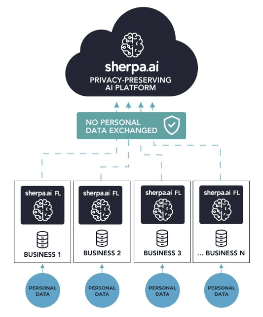
Federated Learning is a Machine Learning paradigm aimed at learning models from decentralized data, such as data located on users’ smartphones, in hospitals, or banks, and ensuring data privacy. This is achieved by training the model locally in each node (e.g., on each smartphone, at each hospital, or at each bank), sharing the model-updated local parameters (not the data) and securely aggregating them to build a better global model.

Traditional Machine Learning requires all the data to be gathered in one single place. In practice, this is often forbidden by privacy regulations. For this reason, Federated Learning is introduced the goal being to learn from a large amount of data, while preserving privacy.

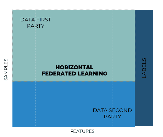
Horizontal Federated Learning is introduced in those scenarios, where data sets share the same feature space (same type of columns) but differ in samples (different rows).

On the one hand, we have this figure which shows the Horizontal Federated Learning (hFL) problem description:

On the other hand, we have the architecture of the solution:

Now that we have the concepts clear, the procedure is the following:

Index

Libraries and data

We are going to use a popular dataset: the framework provides some functions to load the Emnist digits dataset.

import matplotlib.pyplot as plt
import numpy as np
import shfl
import tensorflow as tf
from shfl.auxiliar_functions_for_notebooks.functionsFL import *
from sklearn.metrics import roc_auc_score, f1_score

database = shfl.data_base.Emnist()
train_data, train_labels, test_data, test_labels = database.load_data()

2022-04-25 12:19:15.087501: W tensorflow/stream_executor/platform/default/dso_loader.cc:64] Could not load dynamic library 'libcudart.so.11.0'; dlerror: libcudart.so.11.0: cannot open shared object file: No such file or directory
2022-04-25 12:19:15.087520: I tensorflow/stream_executor/cuda/cudart_stub.cc:29] Ignore above cudart dlerror if you do not have a GPU set up on your machine.

Let's inspect some properties of the loaded data.

print(len(train_data))
print(len(test_data))
print(type(train_data[0]))
train_data[0].shape

240000
40000
<class 'numpy.ndarray'>





(28, 28)

So, as we have seen, our dataset is composed of a set of matrices that are 28 by 28. Before starting with the federated scenario, we can take a look at a sample of the training data.

plt.imshow(train_data[0])

<matplotlib.image.AxesImage at 0x7fbc2d42d7c0>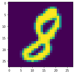

1) Prepare the data and the models for the horizontal federated learning scenario preserving the privacy

1.1) Distribute the datasets in different nodes

We are going to simulate a federated learning scenario with a set of client nodes containing private data, and a central server that will be responsible for coordinating the different clients. But, first of all, we have to simulate the data contained in every client. In order to do that, we are going to use the previously loaded dataset . The assumption in this example is that the data is distributed as a set of independent and identically distributed random variables, with every node having approximately the same amount of data. There are a set of different possibilities for distributing the data. The distribution of the data is one of the factors that can have the most impact on a federated algorithm.

iid_distribution = shfl.data_distribution.IidDataDistribution(database)
nodes_federation, test_data, test_labels = iid_distribution.get_nodes_federation(num_nodes=50, percent=10)

That's it! We have created federated data from the Emnist dataset using 50 nodes and 10 percent of the available data.

A federated learning algorithm is defined by a machine learning model, locally deployed in each node, that learns from the respective node's private data and an aggregating mechanism to _aggregate the different model parameters uploaded by the client nodes to a central node. In this example, we will use a deep learning model using Keras to build it. The framework provides classes on using Tensorflow (see Tensorflow Model) and Keras models in a federated learning scenario, your only job is to create a function acting as model builder. Moreover, the framework provides classes on using pretrained Tensorflow and Keras models (see Pretrained Model). In this example, we will build a Keras learning model.

1.2) The model

For a fair comparison, we are using the same model later for the centralized case.

def emnist_model():
    model = tf.keras.models.Sequential()
    model.add(tf.keras.layers.Conv2D(32, kernel_size=(3, 3), padding='same', activation='relu', strides=1, input_shape=(28, 28, 1)))
    model.add(tf.keras.layers.MaxPooling2D(pool_size=2, strides=2, padding='valid'))
    model.add(tf.keras.layers.Dropout(0.4))
    model.add(tf.keras.layers.Conv2D(32, kernel_size=(3, 3), padding='same', activation='relu', strides=1))
    model.add(tf.keras.layers.MaxPooling2D(pool_size=2, strides=2, padding='valid'))
    model.add(tf.keras.layers.Dropout(0.3))
    model.add(tf.keras.layers.Flatten())
    model.add(tf.keras.layers.Dense(128, activation='relu'))
    model.add(tf.keras.layers.Dropout(0.1))
    model.add(tf.keras.layers.Dense(64, activation='relu'))
    model.add(tf.keras.layers.Dense(10, activation='softmax'))

    loss = tf.keras.losses.CategoricalCrossentropy()
    optimizer = tf.keras.optimizers.RMSprop()
    metrics = [tf.keras.metrics.categorical_accuracy]
    epochs = 1
    batch_size= 32

    return shfl.model.DeepLearningModel(model=model, loss=loss, optimizer=optimizer,
                                        batch_size=batch_size, epochs=epochs, metrics=metrics)

1.3) Preprocessing the data

In addition, we want to normalize the data. The EMNIST dataset is composed by images, and each of the pixels value range between 0 - 255, so in order to normalize the data and set it to a range between 0 - 1, the rescaling is done by dividing the original value with 255.

Moreover, depending on the image type and the model framework, there are sligth adaptations that need to be done. In this case, the image data needs to be reshaped to indicate the model which are the dimensions and the color channels.

Finally, the transforming operations need to be implemented on both trainig data and test data.

A good practice is to define a federated operation that will ensure that the transformation is applied to the federated data in all the client nodes. We want to reshape the data, so we define the following federated transformation.

nodes_federation.apply_data_transformation(normalize_data_image);
nodes_federation.apply_data_transformation(reshape_data_tf);
nodes_federation.apply_data_transformation(cast_to_float);

test_data = np.reshape(test_data, (test_data.shape[0], test_data.shape[1], test_data.shape[2],1))
test_data=test_data/255

1.4) Aggregator

Now, the only missing piece is the aggregation operator. Nevertheless, the framework provides some aggregation operators that we can use. In the following piece of code, we define the federated aggregation mechanism. Moreover, we define the federated government based on the Keras learning model, the federated data, and the aggregation mechanism. The aggregator that we are going to use in this case, is the Federated Averaging defined in the Google's article where the Federated Learning was conceived for the first time.

aggregator = shfl.federated_aggregator.FedAvgAggregator()
federated_government = shfl.federated_government.FederatedGovernment(emnist_model(), nodes_federation, aggregator)

2022-04-25 12:19:18.316911: W tensorflow/stream_executor/platform/default/dso_loader.cc:64] Could not load dynamic library 'libcuda.so.1'; dlerror: libcuda.so.1: cannot open shared object file: No such file or directory
2022-04-25 12:19:18.316929: W tensorflow/stream_executor/cuda/cuda_driver.cc:269] failed call to cuInit: UNKNOWN ERROR (303)
2022-04-25 12:19:18.316944: I tensorflow/stream_executor/cuda/cuda_diagnostics.cc:156] kernel driver does not appear to be running on this host (SH-083-WS): /proc/driver/nvidia/version does not exist
2022-04-25 12:19:18.317115: I tensorflow/core/platform/cpu_feature_guard.cc:151] This TensorFlow binary is optimized with oneAPI Deep Neural Network Library (oneDNN) to use the following CPU instructions in performance-critical operations:  AVX2 FMA
To enable them in other operations, rebuild TensorFlow with the appropriate compiler flags.

2) Run the experiment

2.1) Federated

We are now ready to execute our federated learning algorithm. Each communication round, we will show the loss of the model and the accuracy obtained. Let's see what we obtain:

federated_government.run_rounds(5, test_data, test_labels)

WARNING:tensorflow:5 out of the last 13 calls to <function Model.make_test_function.<locals>.test_function at 0x7fbbcc5268b0> triggered tf.function retracing. Tracing is expensive and the excessive number of tracings could be due to (1) creating @tf.function repeatedly in a loop, (2) passing tensors with different shapes, (3) passing Python objects instead of tensors. For (1), please define your @tf.function outside of the loop. For (2), @tf.function has experimental_relax_shapes=True option that relaxes argument shapes that can avoid unnecessary retracing. For (3), please refer to https://www.tensorflow.org/guide/function#controlling_retracing and https://www.tensorflow.org/api_docs/python/tf/function for  more details.
WARNING:tensorflow:5 out of the last 13 calls to <function Model.make_test_function.<locals>.test_function at 0x7fbbe41353a0> triggered tf.function retracing. Tracing is expensive and the excessive number of tracings could be due to (1) creating @tf.function repeatedly in a loop, (2) passing tensors with different shapes, (3) passing Python objects instead of tensors. For (1), please define your @tf.function outside of the loop. For (2), @tf.function has experimental_relax_shapes=True option that relaxes argument shapes that can avoid unnecessary retracing. For (3), please refer to https://www.tensorflow.org/guide/function#controlling_retracing and https://www.tensorflow.org/api_docs/python/tf/function for  more details.
Evaluation in round 0:

Collaborative model test -> loss: 1.9170536994934082  categorical_accuracy: 0.6445249915122986

Evaluation in round 1:

Collaborative model test -> loss: 1.0888532400131226  categorical_accuracy: 0.7615249752998352

Evaluation in round 2:

Collaborative model test -> loss: 0.737216055393219  categorical_accuracy: 0.8216500282287598

Evaluation in round 3:

Collaborative model test -> loss: 0.5709713697433472  categorical_accuracy: 0.8522999882698059

Evaluation in round 4:

Collaborative model test -> loss: 0.48093652725219727  categorical_accuracy: 0.8719750046730042

It is really interesting to see how the accuracy improves when the number of rounds increases. This is due to the fact that the averaged parameters are being updated in the server in each round and sent back to the nodes. Upon receiving these parameters, the local nodes initializes their models with the received weights, and train for some numbers of iterations. This tends to improve the training.

First of all, we need to compute the results using the model of the federated case in order to compare it to the local and centralized case.

federated_model = federated_government._server._model
predictions_fed = federated_model.predict(test_data)

accuracy_fed = accuracy(predictions_fed, test_labels)

After that, we replicate the model for the centralized case and we feed all the data to it. For this purpose, we need to reshape and include the operations we did before to the training data, as this operations were only applied to the node's data inside the federation.

n_classes = 10
train_data = np.reshape(train_data, (train_data.shape[0], train_data.shape[1], train_data.shape[2],1))
train_data=train_data.astype(np.float32)
train_data = (train_data / 255)

2.2) Local (using the data of the first node)

For the local test, we implemented a method to obtain the node's data experimentally. However, THIS IS NOT APPLICABLE IN A REAL CASE OR IN THE PLATFORM AND IT IS MADE FOR TESTING PURPOSES ONLY. All of these notebooks are made with an experimental implementation of the code where security measures are bypassed for explainability reasons.

for i in nodes_federation[0]._private_data:
    local_data = nodes_federation[0]._private_data[i].data
    local_label = nodes_federation[0]._private_data[i].label

We create the same model and fit the available data the local scenario. We need to predict the test data with the local model so as to obtain the probabilities of belonging to each of the classes.

model_loc = emnist_model()
model_loc.train(local_data, local_label)

predictions_loc = model_loc.predict(test_data)

accuracy_loc = accuracy(predictions_loc, test_labels)

2.3) Centralized (data joined with any kind of privacy)

The centralized data represents a node that has the whole dataset, joined without any kind of privacy. In principle, this will imply a better accuracy but, for sure, this can not happen in a real world scenario, where the data are dispersed over different organizations under the protection of privacy restrictions. We will load the centralized data, joining the two datasets.

We create the same model and fit the available data the centralized scenario. We need to predict the test data with the local model so as to obtain the probabilities of belonging to each of the classes.

model_cent = emnist_model()
model_cent.train(train_data, train_labels)

predictions_cent = model_cent.predict(test_data)

accuracy_cent = accuracy(predictions_cent, test_labels)

After the training process, we can check the accuracy of the models.

2.4) Comparison

With the previous obtained results, we can extract the following figure:

values=[round(accuracy_loc, 3), round(accuracy_fed, 3), round(accuracy_cent, 3)]
titles=['Local', 'Federated', 'Centralized']
colors=['blue', 'green', 'red']
plot_all_metric(values, "Accuracy", titles, colors)

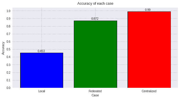
Even though the accuracy is good to understand the performance of a model, by itself is not a good metric to compare different models. For this reason we are going to calculate the ROC AUC scores for these 3 models:

2.4.1) ROC curve

To calculate the ROC curve in a multilabel environment, instead of plotting each of the labels, it is visually more appealing to calculate the average of them and show it. There are few strategies to consider when calculating this value and in our case the micro-average is computed, which is the sum of all true positives and divides by the sum of all true positives plus the sum of all false positives. So basically you divide the number of correctly identified predictions by the total number of predictions.

Finally, these results are plotted to visually see the difference between the 2 classifiers, taking into account that the centralized case is hypothetical, it vulnerates privacy laws as all the data needs to be gathered in one place, something imposible in most cases.

values=[predictions_loc, predictions_fed, predictions_cent]
titles=['Local', 'Federated', 'Centralized']
colors=['blue', 'green', 'red']
linestyle=[':','-','-.']

plot_all_roc_curves(test_labels, values, titles, colors, linestyle)

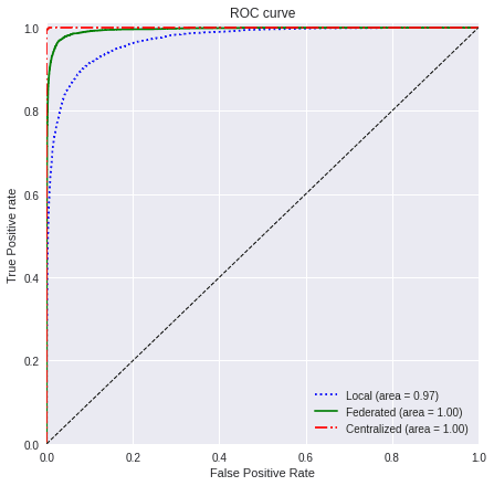
Looking at the final results, it is clear that the performance of the federated model is really close to the centralized one, being the best choice overall due to it's privacy preserving mechanisms and adaptability to real world scenarios.

However, only calculating a metric could make the evaluation a little bit biased, so it is recommendable to use another comparison value just to be sure.

2.4.2) F1-Score

Another metric used is the F1 score, which seeks the balance between precision and recall values. This metric will allow us to estimate performance in another way and better compare the results.

n_classes=10

values_f1_fed = predictions_fed.argmax(axis=-1)
values_f1_fed = np.eye(n_classes)[values_f1_fed]

values_f1_cent = predictions_cent.argmax(axis=-1)
values_f1_cent = np.eye(n_classes)[values_f1_cent]

values_f1_loc = predictions_loc.argmax(axis=-1)
values_f1_loc = np.eye(n_classes)[values_f1_loc]


score_fed_f1 = f1_score(test_labels, values_f1_fed, average='macro')
score_cent_f1 = f1_score(test_labels, values_f1_cent, average='macro')
score_loc_f1 = f1_score(test_labels, values_f1_loc, average='macro')


values=[round(score_loc_f1, 3), round(score_fed_f1, 3), round(score_cent_f1, 3)]
titles=['Local', 'Federated', 'Centralized']
colors=['blue', 'green', 'red']
plot_all_metric(values, "F1-Score", titles, colors)

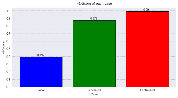
With both evaluations, it is clear that horizontal Federated Learning is a proper alternative to the centralized model, not only for fullfilling the privacy requirements by law, but also due to it's high performance that benefits all the participating nodes in the process.