Differential privacy: composition concepts

In this notebook we explain more advanced Differential Privacy (DP) concepts, such as composition theorems and how to use them in the Sherpa.ai Federated Learning and Differential Privacy Framework. Before diving in, we recommend reading section 3.5 of The Algorithmic Foundations of Differential Privacy and everything related to Privacy Filters from the paper Privacy Odometers and Filters: Pay-as-you-Go Composition.

Index

1) Composition theorems

A great property of DP is that private mechanisms can be composed while preserving DP. The new values of $\epsilon$ and $\delta$ can be computed according to the composition theorems. Before the composition theorems are provided, we are going to state an experiment with an adversarial, which proposes a composition scenario for DP.

Composition experiment $b \in \{ 0,1 \}$ for adversary $A$ with a given set, $M$, of DP mechanisms:

For $i=1,\dots,k$:

1. $A$ generates two neighbouring databases $x_i^0$ and $x_i^1$ and selects a mechanism $\mathcal{M}_i$ from $M$.
2. $A$ receives the output $y_i \in \mathcal{M}_i(x_i^b)$, which is stored in $V^b$

Note that the adversary is stateful, that is, it stores the output in each iteration and selects the DP mechanism based on the observed outputs.

Note on neighboring databases:

It is important to know that when it comes to numeric databases, such as two arrays, $A=[1,2,3,4]$ and $B=[1,2,5,8]$ (which is the main use case for the Sherpa.ai Federated Learning and Differential Privacy Framework). They are neighboring databases if they differ in only one component, up to as much as 1 (the must have the same length), therefore A and B aren't neighboring databases but, $C=[1,28,91]$ and $D=[2,28,91]$ are.

from shfl.private.node import DataNode
from shfl.differential_privacy.mechanism import LaplaceMechanism, GaussianMechanism
from math import log, exp
import numpy as np

def run_composition_experiment(M, db_storage, secret):
    # Number of runs equals the number of mechanisms provided
    k = len(M)
    
    # Adversary's view in experiment 1
    A_view1 = np.empty(shape=(k,))
    # Adversary's view in experiment 2
    A_view2 = np.empty(shape=(k,))

    # Neighboring databases are created
    db1 = "db1"
    db2 = "db2"
    db_storage.set_private_data(name=db1, data=secret)
    db_storage.set_private_data(name=db2, data=secret+1)

    # In the following loop, we reproduce both experiments for b=0 and for b=1
    for i in range(k):
        # The adversarial selects the dp-mechanism
        db_storage.configure_data_access(db1, M[i])
        db_storage.configure_data_access(db2, M[i])
        # The outputs are stored in the adversary's view in each experiment
        A_view1[i] = db_storage.query(db1)
        A_view2[i] = db_storage.query(db2)
    
    return A_view1, A_view2

2022-03-23 12:53:25.777868: W tensorflow/stream_executor/platform/default/dso_loader.cc:64] Could not load dynamic library 'libcudart.so.11.0'; dlerror: libcudart.so.11.0: cannot open shared object file: No such file or directory
2022-03-23 12:53:25.777884: I tensorflow/stream_executor/cuda/cudart_stub.cc:29] Ignore above cudart dlerror if you do not have a GPU set up on your machine.

As you can see in the following piece of code, privacy is preserved, as it is not possible to tell in which database the secret is stored. However, if this experiment is run enough times, the probability of telling the difference increases, so what is the privacy budget spent in these experiments? This is the fundamental question that composition theorems answer.

# Setup storage for all databases
db_storage = DataNode()

# List of DP-mechanisms
M = [LaplaceMechanism(1, epsilon=0.5), 
     LaplaceMechanism(1, epsilon=1), 
     GaussianMechanism(1, epsilon_delta=(0.5, 0.01))]

A_view1, A_view2 = run_composition_experiment(M, db_storage, 1)
    
print("Adversary's view from Experiment 1: {}, mean: {}".format(A_view1, np.mean(A_view1)))
print("Adversary's view from Experiment 2: {}, mean: {}".format(A_view2, np.mean(A_view2)))

Adversary's view from Experiment 1: [ 1.30650244 -1.15824919  4.93544852], mean: 1.694567257183766
Adversary's view from Experiment 2: [2.04486821 2.17145275 2.62126022], mean: 2.279193724627244

As expected, if the experiment is carried on for enough rounds, we can determine in which database the secret is stored.

# Setup storage for all databases
db_storage = DataNode()

# List of DP-mechanisms
M = [LaplaceMechanism(1, epsilon=0.5), 
     LaplaceMechanism(1, epsilon=1), 
     GaussianMechanism(1, epsilon_delta=(0.5, 0.01))]*1000

A_view1, A_view2 = run_composition_experiment(M, db_storage, 1)
    
print("Adversary's view from Experiment 1 mean: {}".format(np.mean(A_view1)))
print("Adversary's view from Experiment 2 mean: {}".format(np.mean(A_view2)))

Adversary's view from Experiment 1 mean: 1.0096424469891259
Adversary's view from Experiment 2 mean: 1.9420186200234533

1.1) Basic composition theorem

The first and most basic theorem that can be employed for composition is the Basic Composition Theorem. The composition of a sequence $\{\mathcal{M}_k\}$ of ($\epsilon_i, \delta_i$)-differentially private mechanisms under the Composition experiment with $M=\{\mathcal{M}_k\}$, is ($\sum_{i=1}^{k} \epsilon_i, \sum_{i=1}^{k} \delta_i$)-differentially private.

In other words, it states that the resulting privacy budget is the sum of the privacy budget spent in each access. Therefore, the budget expended in the previous experiment was:

epsilon_delta_access = [m.epsilon_delta for m in M]
epsilon_spent, delta_spent = map(sum, zip(*epsilon_delta_access))
print("{} epsilon was spent".format(epsilon_spent))
print("{} delta was spent".format(delta_spent))

2000.0 epsilon was spent
9.999999999999831 delta was spent

The main disadvantage of this theorem is that it assumes a worst case scenario. A better bound can be stated using the Advanced Composition Theorem.

1.2) Advanced composition theorem

For all $\epsilon, \delta, \delta' \geq 0$ the composition of a sequence $\{\mathcal{M}_k\}$ of ($\epsilon, \delta$)-differentially private mechanisms under the Composition experiment with $M=\{\mathcal{M}_k\}$, satisfies ($\epsilon', \delta''$)-DP with:

In other words, for a small sacrifice $\delta$' in the global $\delta$ spent, we can achieve a better bound for the global $\epsilon$ spent. However, the theorem assumes that the same DP mechanism is used in each access:

from math import sqrt

# Basic theorem computations
def basic_theorem_expense(epsilon, delta, k):
    epsilon_spent = k*epsilon
    delta_spent = k*delta
    return epsilon_spent, delta_spent

# Advanced theorem computations
def advanced_theorem_expense(epsilon, delta, delta_sacrifice, k):
    epsilon_spent = sqrt(2*k*log(1/delta_sacrifice)) + k * epsilon * (exp(epsilon) - 1)
    delta_spent = k*delta + delta_sacrifice
    return epsilon_spent, delta_spent


epsilon = 0.5
delta = 0
k = 3
delta_sacrifice = 0.1

basic = basic_theorem_expense(epsilon, delta, k)
advanced = advanced_theorem_expense(epsilon, delta, delta_sacrifice, k)

print("Epsilon: {} vs {} (basic theorem vs advanced theorem) ".format(basic[0], advanced[0]))
print("Delta: {} vs {} (basic theorem vs advanced theorem) ".format(basic[1], advanced[1]))

Epsilon: 1.5 vs 4.690004094900031 (basic theorem vs advanced theorem) 
Delta: 0 vs 0.1 (basic theorem vs advanced theorem) 

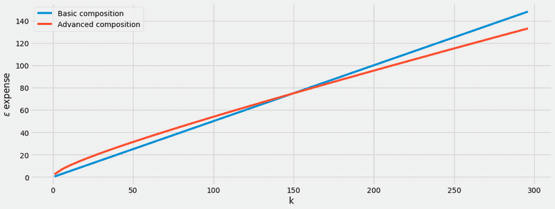
But wait, if the epsilon spent is worse with the new theorem, is it useless? Of course not, let's see what happens when we increase the number of iterations:

epsilon = 0.5
delta = 0
k = 350
delta_sacrifice = 0.1

basic = basic_theorem_expense(epsilon, delta, k)
advanced = advanced_theorem_expense(epsilon, delta, delta_sacrifice, k)

print("Epsilon: {} vs {} (basic theorem vs advanced theorem) ".format(basic[0], advanced[0]))
print("Delta: {} vs {} (basic theorem vs advanced theorem) ".format(basic[1], advanced[1]))

Epsilon: 175.0 vs 153.67357054267973 (basic theorem vs advanced theorem) 
Delta: 0 vs 0.1 (basic theorem vs advanced theorem) 

So, we can conclude that the benefits of the advanced theorem are only noticeable when the number of mechanism accesses is huge. In particular, we can observe that for values of $k$ close to 150 (and $\delta=0.1$), the theorems are almost identical.

import matplotlib.pyplot as plt

plt.style.use('fivethirtyeight')

fig, ax = plt.subplots(nrows=1, ncols=1, figsize=(16,6))
k_values = np.arange(1, 300, 5)
ax.plot(k_values, [basic_theorem_expense(epsilon, delta, k)[0] for k in k_values], label = "Basic composition")  
ax.plot(k_values, [advanced_theorem_expense(epsilon, delta, delta_sacrifice, k)[0] for k in k_values], label = "Advanced composition")   
ax.set_xlabel('k')
ax.set_ylabel('$\epsilon$ expense')

plt.legend(title = "", loc="upper left")
plt.show()

While composition theorems are quite useful, they require some parameters to be defined upfront, such as the number of mechanisms to be composed. Therefore, no intermediate result can be observed and the privacy budget can be wasted. In such situations, a more fine grained composition technique, which allows to observe the result of each mechanism to be observed without compromising the privacy budget spent, is required. In order to remove some of the stated constraints, a more flexible experiment of composition can be introduced:

2) Adaptive composition experiment $b \in \{ 0,1 \}$ for adversary $A$

For $i=1,\dots,k$:

1. $A$ generates two neighboring databases $x_i^0$ and $x_i^1$ and selects a mechanism $\mathcal{M}_i$ that is ($\epsilon_i, \delta_i$)-differentially private.
2. $A$ receives the output $y_i \in \mathcal{M}_i(x_i^b)$

Note that in these situations, the $\epsilon_i$ and $\delta_i$ of each mechanism is adaptively selected, based on the outputs of previous iterations.

Now we introduce the privacy filter, which can be used to guarantee with high probability in the Adaptive Composition experiments, the stated privacy budget $\epsilon_g$ is never exceeded. Privacy filters have similar composition theorems to those mentioned previously:

2.1) Basic composition for privacy filters

For any $\epsilon_g, \delta_g \geq 0,\$ $\texttt{COMP}_{\epsilon_g, \delta_g}$ is a valid Privacy Filter:

2.2) Advanced composition for privacy filters

We define $\mathcal{K}$ as follows:

with $H = \frac{\epsilon_g^2}{28.04 \ln(1/\delta_g)}$

Then $\texttt{COMP}_{\epsilon_g, \delta_g}$ is a valid Privacy Filter for $\delta_g \in (0, 1/e)$ and $\epsilon_g > 0$, where:

The value of $\mathcal{K}$ might be strange at first sight, however, if we assume $\epsilon_j=\epsilon$ for all $j$, it remains:

which is quite similar to the expression given in the Advanced Composition Theorem.

3) Privacy filters in the Sherpa.ai Federated Learning and Differential Privacy Framework

This framework implements Privacy Filters and transparently applies both theorems stated before, so that there is no need to constantly check which theorem ensures a better ($\epsilon, \delta$) expense. When the fixed privacy budget is surpassed, an exception ExceededPrivacyBudgetError is raised. The following example shows two equivalent implementations of the Adaptive Composition experiment, stated before.

from shfl.private.node import DataNode
from shfl.differential_privacy.composition import AdaptiveDifferentialPrivacy
from shfl.differential_privacy.composition import ExceededPrivacyBudgetError
from shfl.differential_privacy.mechanism import LaplaceMechanism
import numpy as np


def run_adaptive_comp_experiment_v1(global_eps_delta, eps_delta_access):
    # Define a place to store the data
    node_single = DataNode()

    # Store the private data
    node_single.set_private_data(name="secret", data=np.array([1]))

    # Choose your favorite differentially_private_mechanism
    dpm = LaplaceMechanism(sensitivity=1, epsilon=eps_delta_access)

    # Here we are specifying that we want to use composition theorems for Privacy Filters
    # DP mechanis
    default_data_access = AdaptiveDifferentialPrivacy(global_eps_delta, mechanism=dpm)
    node_single.configure_data_access("secret", default_data_access)

    result_query = []
    while True:
        try:
            # Queries are performed using the Laplace mechanism
            result_query.append(node_single.query(private_property="secret"))
        except ExceededPrivacyBudgetError:
            # At this point we have spent the entiry privacy budget
            break       
    
    return result_query

The second implementation copies the same code, with a slight variation on the procedure of specifying the Differential Privacy mechanism.

def run_adaptive_comp_experiment_v2(global_eps_delta, eps_delta_access):
    node_single = DataNode()

    node_single.set_private_data(name="secret", data=np.array([1]))

    dpm = LaplaceMechanism(sensitivity=1, epsilon=eps_delta_access)

    default_data_access = AdaptiveDifferentialPrivacy(global_eps_delta)
    node_single.configure_data_access("secret", default_data_access)

    result_query = []
    while True:
        try:
            # DP mechanism is specified at time of query, in this case the Laplace mechanism
            # if no mechanism is specified an exception is raised
            result_query.append(node_single.query(private_property="secret", mechanism=dpm))
        except ExceededPrivacyBudgetError:
            # At this point we have spent the entiry privacy budget
            break         
    
    return result_query

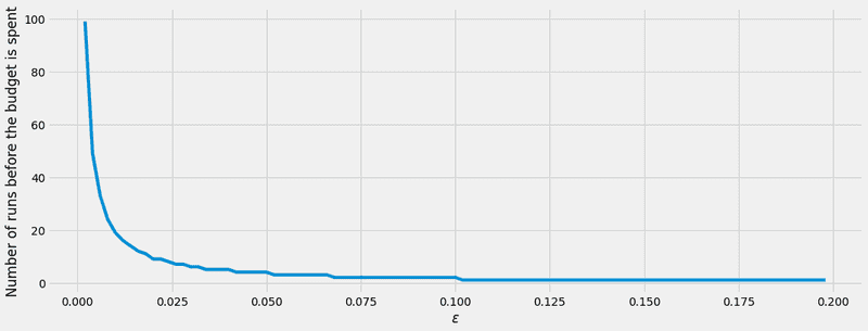
Either way, we test the Laplace mechanism in this experiment to test the privacy budget. In the following plot, we can see that the privacy budget is spent significantly faster, as $\epsilon$ moves away from 0, in other words, when the privacy is lower.

global_epsilon_delta = (2e-1, 2e-30)  
epsilon_values = np.arange(2e-3, 2e-1, 2e-3)
plt.style.use('fivethirtyeight')

fig, ax = plt.subplots(nrows=1, ncols=1, figsize=(16,6))
y_axis=[len(run_adaptive_comp_experiment_v1(global_epsilon_delta, e)) for e in epsilon_values] 
ax.plot(epsilon_values, y_axis)  
ax.set_xlabel('$\epsilon$')
ax.set_ylabel('Number of runs before the budget is spent')

plt.show()

Note:

These experiments are run with the same DP mechanism, for the sake of simplification. If you want to access your data with a different DP mechanism, we recommend using a schema similar to the one shown in the function run_adaptive_comp_experiment_v2.