Encapsulate a custom model

⚠

Please note that these tutorials refer to a deprecated version of the platform. The current version of the platform, which is not publicly available, has a more advanced architecture and provides a wider range of functionalities. These tutorials are only for illustrative purposes and showcase a limited number of the platform’s capabilities.

# Federated models: encapsulate a custom model in Sherpa.ai Federated Learning and Differential Privacy Framework

This notebook covers the problem of encapsulating a custom machine learning model into the Sherpa.ai Federated Learning and Differential Privacy Framework for experimentation in the federated configuration. In this case, we will create a learning model from scratch and show how to make it interact with the Sherpa.ai Federated Learning and Differential Privacy Framework. For the sake of simplicity, a two-feature case of linear regression is considered, since an explicit formula for the minimization of the object function is available (see the Introduction to statistical learning, Section 3.1). For completeness, we assess the accuracy in a federated learning context, and we address the privacy level needed, in terms of sampling the sensitivity of our model for application of Differential Privacy.

In order to make our model interact with the framework, we will simply need to define:

The data
The model

In the following, each step is described for the case of a 2D linear regression model.

Index

1) The data

A method that returns training, test, and validation data needs to be provided, wrapping it in the class data_base. Typically, existing data is used. However, in this example, a series of 2D points is created for simplicity:

import numpy as np
import matplotlib.pyplot as plt

import shfl
from shfl.auxiliar_functions_for_notebooks.functionsFL import *
from shfl.data_base.data_base import WrapLabeledDatabase
from shfl.private.reproducibility import Reproducibility

# Ensure reproducible results
Reproducibility(123)

def generate_data():
    size_data=100
    beta0=10
    beta1=2
    scale=10

    data=np.random.randint(low=0, high=100, size=size_data, dtype='l')
    labels=beta0 + beta1*data + np.random.normal(loc=0.0, scale=scale, size=len(data))
    
    return data, labels

# Create database:
data, labels = generate_data()
database = WrapLabeledDatabase(data, labels)
train_data, train_labels, test_data, test_labels = database.load_data()
print('Length of the generated training data=', len(train_data))
print('Length of the generated test data=', len(test_data))

2022-03-24 17:47:34.915080: W tensorflow/stream_executor/platform/default/dso_loader.cc:64] Could not load dynamic library 'libcudart.so.11.0'; dlerror: libcudart.so.11.0: cannot open shared object file: No such file or directory
2022-03-24 17:47:34.915096: I tensorflow/stream_executor/cuda/cudart_stub.cc:29] Ignore above cudart dlerror if you do not have a GPU set up on your machine.


Length of the generated training data= 80
Length of the generated test data= 20

2) The model

Now, we just need to define the model, which needs to be wrapped in the class TrainableModel. Abstract methods from class TrainableModel need to be defined, i.e., we must provide methods for train, predict, evaluate, performance, get_parameters, and set_parameters. For the evaluate method, we choose the Root Mean Squared and the Mean Absolute Percentage errors as performance metrics. A possible implementation is the following:

from shfl.model import TrainableModel
from sklearn.metrics import r2_score

class LinearRegression2D(TrainableModel):
    
    def __init__(self, beta0=0.0, beta1=0.0):
        self._beta0=beta0
        self._beta1=beta1
        
    def train(self, data, labels,**kwargs):
        """
        In the case of 2D linear regression, a closed formula can be used.
        """
        data_mean=np.mean(data)
        labels_mean=np.mean(labels)
        beta1=np.sum( np.multiply((data-data_mean), (labels-labels_mean)) ) / np.sum( np.square((data-data_mean)) )
        beta0=labels_mean - beta1*data_mean
        self._beta0=beta0
        self._beta1=beta1
        
    def predict(self, data):
        y_predicted=self._beta0 + self._beta1 * data
        
        return(y_predicted)
    
    def evaluate(self, data, labels):
        """
        Add all the metrics to evaluate the performance here. 
        """
        prediction=self.predict(data)
        error=np.square(labels - prediction)
        RMSE=('RMSE', np.sqrt(error.mean()))
        R2=('R2', r2_score(labels, prediction))
        metric = [RMSE,R2]
        return metric
    
    def performance(self, data, labels):
        
        return self.evaluate(data, labels)[0]

    def get_model_params(self):
        return np.asarray((self._beta0, self._beta1))
    
    def set_model_params(self, params):
        self._beta0=params[0]
        self._beta1=params[1]

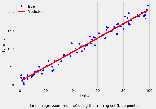
We can graphically check that our implementation is correct by training the model on the centralized data:

# Plot the regression over the train data:
LR=LinearRegression2D()
LR.train(data=train_data, labels=train_labels)
print("Regression coefficients: " + str((LR._beta0, LR._beta1)))

# Reference centralized (non federate) model:
print("Performance metrics on test data: ", end='')

for metric in LR.evaluate(data=test_data, labels=test_labels):
    print(metric[0]+": "+str(metric[1]), end='  ')


plt.style.use('fivethirtyeight')
fig, ax=plt.subplots(figsize=(9,6))
ax.plot(train_data, train_labels, 'bo', label="True")
ax.plot(train_data, LR.predict(data=train_data), label="Predicted", color="red")
ax.set_xlabel('Data')
ax.set_ylabel('Labels')
plt.legend(title="")
label="Linear regression (red line) using the training set (blue points)"
ax.text((train_data.max()+train_data.min())/2, -60, label, ha='center')

plt.show()

Regression coefficients: (9.254134370807037, 1.997846243301223)
Performance metrics on test data: RMSE: 10.496223822795809  R2: 0.9656486050932186

png

3) Run the federated learning experiment

After defining the data and the model, we are ready to run our model in a federated configuration. We distribute the data over the nodes, assuming the data is IID. Next, we define the aggregation of the federated outputs to be the average. In this case, we set the number of rounds to n=1, since no iterations are needed in this specific case of 2D linear regression. It can be observed that the performance of the federated global model is generally superior, with respect to the performance of each node, thus, the federated learning approach proves to be beneficial. Moreover, the federated global model exhibits comparable performance to that of the centralized one (see the previous cell).

# Create the IID data: 
iid_distribution=shfl.data_distribution.IidDataDistribution(database)
nodes_federation, test_data, test_label = iid_distribution.get_nodes_federation(num_nodes=12, percent=100)
print(type(nodes_federation))
print(nodes_federation.num_nodes())

# Define a model builder: 
def model_builder():
    model=LinearRegression2D()
    return model

# Run the algorithm:
aggregator = shfl.federated_aggregator.FedAvgAggregator()
federated_government = shfl.federated_government.FederatedGovernment(model_builder(), nodes_federation, aggregator)

federated_government.run_rounds(n_rounds=1, test_data=test_data, test_label=test_label)

<class 'shfl.private.federated_operation.NodesFederation'>
12
Evaluation in round 0:

Collaborative model test -> RMSE: 10.4101195237816  R2: 0.9662098871063219

4) Add differential privacy

We wish to add Differential Privacy to our federated learning experiment, and assess its effect on the quality of the global model. In the following, it is shown how to perform that by easy steps using Sherpa.ai framework. As shown below, by selecting a sensitivity we are ready to run the private federated experiment using the desired differential privacy mechanism.

4.1) Model's sensitivity

In the case of applying the Laplace privacy mechanism, the noise added has to be of the same order as the sensitivity of the model's output (the values of the intercept and slope in our 2D linear regression). In the general case, the model's sensitivity might be difficult to compute analytically. An alternative approach is to attain random differential privacy through a sampling over the data (see Rubinstein 2017). That is, instead of computing the global sensitivity $\Delta f$ analytically, we compute an empirical estimation of it by sampling over the dataset. The framework provides a method for sampling the sensitivity.

In order to carry out this approach, we need to specify a distribution of the data to sample from. Generally, this requires previous knowledge and/or model assumptions. However, we may assume that the data distribution is uniform and avoid specific assumptions. We define our class of ProbabilityDistribution that uniformly samples over a data-frame. Moreover, we assume that we do have access to a set of data (this can be thought of, for example, as a public data set). In this example, we generate new data for sampling:

class UniformDistribution(shfl.differential_privacy.ProbabilityDistribution):
    """
    Implement Uniform Distribution over real data
    """
    def __init__(self, sample_data):
        self._sample_data=sample_data

    def sample(self, sample_size):
        row_indices=np.random.randint(low=0, 
                                        high=self._sample_data.shape[0], 
                                        size=sample_size, 
                                        dtype='l')
        
        return self._sample_data[row_indices, :]
    
# Generate new data for sampling: 
data, labels = generate_data()
database=WrapLabeledDatabase(data, labels)
data_sample, labels_sample, _, _ = database.load_data()
sample_data = np.zeros((len(data_sample), 2))
sample_data[:,0] = data_sample
sample_data[:,1] = labels_sample

The class SensitivitySampler implements the sampling, given a query (i.e, the learning model itself, in this case). We only need to add the __call__ method to our model since it is required to be callable. We choose the sensitivity norm to be the $L_1$ norm and we apply the sampling. Typically, the value of the sensitivity is influenced by the size of the sampled data: the higher, the more accurate the sensitivity. Indeed, by increasing the size of the sampled data, the sensitivity decreases, as shown below:

from shfl.differential_privacy import SensitivitySampler
from shfl.differential_privacy import L1SensitivityNorm

class LinearRegression2DSample(LinearRegression2D):
    
    def __call__(self, data_array):
        data=data_array[:, 0]
        labels=data_array[:, 1]
        train_model=self.train(data, labels)
        
        return np.asarray(self.get_model_params())

distribution = UniformDistribution(sample_data)
sampler = SensitivitySampler()

n_data_size = 10
max_sensitivity, mean_sensitivity = sampler.sample_sensitivity(LinearRegression2DSample(), 
                                                               L1SensitivityNorm(), 
                                                               distribution, 
                                                               n_data_size=n_data_size, 
                                                               gamma=0.05)
print("Sampled max sensitivity: " + str(max_sensitivity))
print("Sampled mean sensitivity: " + str(mean_sensitivity))

Sampled max sensitivity: 19.838194824524173
Sampled mean sensitivity: 2.529693294269198

n_data_size=500
max_sensitivity, mean_sensitivity=sampler.sample_sensitivity(LinearRegression2DSample(), 
                                                             L1SensitivityNorm(), 
                                                             distribution, 
                                                             n_data_size=n_data_size, 
                                                             gamma=0.05)
print("Sampled max sensitivity: " + str(max_sensitivity))
print("Sampled mean sensitivity: " + str(mean_sensitivity))

Sampled max sensitivity: 0.23830351791791538
Sampled mean sensitivity: 0.042064154999351615

Unfortunately, sampling over a dataset involves the training of the model on two datasets differing in one entry, at each sample. Thus, in general, this procedure might be computationally expensive (e.g., in the case of training a deep neural network).

4.2) Run the federated learning experiment with differential privacy

At this stage we are ready to add a layer of DP to our federated learning model. We will apply the Laplace mechanism, assuming the sensitivity of our model is that which was obtained from the previous sampling. The Laplace mechanism provided by the Sherpa.ai Federated Learning and Differential Privacy Framework is then assigned as the private access type to the model parameters of each client in a new FederatedGovernment object. This results in an $\epsilon$ -differentially private FL model. For example, by choosing the value $\epsilon=0.5$ , we can run the FL experiment with DP:

from shfl.differential_privacy import LaplaceMechanism

params_access_definition=LaplaceMechanism(sensitivity=max_sensitivity, epsilon=0.5)
nodes_federation.configure_model_params_access(params_access_definition)
federated_governmentDP=shfl.federated_government.FederatedGovernment(
    model_builder(), nodes_federation, aggregator)

federated_governmentDP.run_rounds(n_rounds=1, test_data=test_data, test_label=test_labels)

Evaluation in round 0:

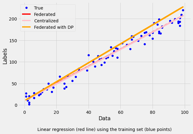
Collaborative model test -> RMSE: 11.438958902181435  R2: 0.9592008410638743

In the above example, we saw that the performance of the model deteriorated slightly, due to the addition of differential privacy. It must be noted that each run involves a different random noise added by the differential privacy mechanism. However, in general, privacy increases at the expense of accuracy (i.e., for smaller values of $\epsilon$ ). Let's see how did the linear regressions adjusted to the actual data.

5) Comparing the metrics

Now that we have all the models, let's do the metrics calculations:

from shfl.auxiliar_functions_for_notebooks.functionsFL import *
import matplotlib.pyplot as plt

fed_model = federated_government._server._model
predictions_fed_train = fed_model.predict(train_data)
evaluation_fed = fed_model.evaluate(train_data, train_labels)


dp_model = federated_governmentDP._server._model
predictions_dp_train = dp_model.predict(train_data)
evaluation_dp = dp_model.evaluate(train_data, train_labels)


predictions_cent_train = LR.predict(train_data)
evaluation_cent = LR.evaluate(train_data, train_labels)

Then we plot the training results to see how the different models adapted to the values:

plt.style.use('fivethirtyeight')
fig, ax=plt.subplots(figsize=(9,6))
ax.plot(train_data, train_labels, 'bo', label="True")
ax.plot(train_data, predictions_fed_train, label="Federated", color="red")
ax.plot(train_data, predictions_cent_train, label="Centralized", color="pink")
ax.plot(train_data, predictions_dp_train, label="Federated with DP", color="orange")
ax.set_xlabel('Data')
ax.set_ylabel('Labels')
plt.legend(title="")
label="Linear regression (red line) using the training set (blue points)"
ax.text((train_data.max()+train_data.min())/2, -60, label, ha='center')

plt.show()

png

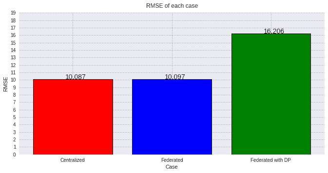
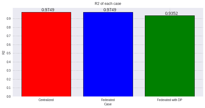
Now, let's go with the result metrics. We are evaluating the Root Mean Squared Error and then, the R2 coefficient, and plotting the values from all the models:

values=[round(evaluation_cent[0][1], 3), round(evaluation_fed[0][1], 3), round(evaluation_dp[0][1], 3)]
titles=['Centralized', 'Federated', 'Federated with DP']
colors=['red', 'blue', 'green']
plot_all_RMSE(values, titles, colors, 20)

png

values=[round(evaluation_cent[1][1], 4), round(evaluation_fed[1][1], 4), round(evaluation_dp[1][1], 4)]
plot_all_R2(values, titles, colors)

png

As expected, the federated case behaves much alike the centralized model, but when adding a high privacy $\epsilon$ coefficient the performance is slightly hindered.