Horizontal Federated Learning case: Fraud detection
In this notebook, we provide an example of how to perform an Horizontal Federated Learning (HFL) experiment with the help of the Sherpa.ai Federated Learning framework. We simulate a scenario, where we have a federation of banks, which owns different rows of a dataset previously preprocessed. The final goal is to predict whether a transaction is fraudulent or not. It is important that credit card companies are able to recognize fraudulent credit card transactions so that customers are not charged for items that they did not purchase. If successful, the federated solution can improve the efficacy of fraudulent transaction alerts for millions of people around the world, helping hundreds of thousands of businesses reduce their fraud loss and increase their revenue.
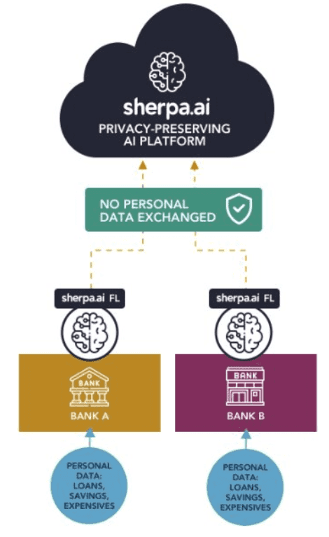
The architecture of the solution that we propose with the Sherpa.ai platform is the next one:

To set up the federated learning experiment we will show the simple steps for loading the dataset and distribute it to a federated network of clients, and we will define the model that will be trained in the federated learning rounds.
Moreover, we will compare a local node's execution with only it's own data, the hipothetical case where all the data is centralized and the federated scenario to check the obtained models' performances against the testing data. Finally, we will further discuss the viability of horizontal Federated Learning.
Once that we have a general overview of our problem, the procedure is the following:
Index
0) Libraries and data
We load all the functions that we are going to use to develop our experiment:.
import matplotlib
matplotlib.use('Agg')

import pandas as pd
import shfl
from shfl.auxiliar_functions_for_notebooks.preprocessing import label_encoder
from shfl.data_base.data_base import WrapLabeledDatabase
from shfl.data_base.data_base import split_train_test
from shfl.auxiliar_functions_for_notebooks.functionsFL import *
pd.set_option("display.max_rows", 30, "display.max_columns", None)
from shfl.private.reproducibility import Reproducibility
Reproducibility(987)
As we have mentioned, the dataset is anonymized and correspond to two different banks. The first half of the dataset correspond to the first bank and the second half to the second. Of course, in a real-world scenario, datasets can not be joined, but for the sake of simplicity, we will perform a simulation, where:
- The federated case correspond to the case where the banks collaborate privately with a view to improve the predictions.
- The centralized case correspond to the case of the data joined without privacy. This will show us the results that we would obtain if the banks shared its private data between them (forbidden by law).
- The local cases correspond to the cases there the banks try to perform a prediction with its own data respectively. This means, that the data are siloed.
We show then the whole data that we are going to be working with:
dataframe = pd.read_csv('fraud_detection_bank_dataset.csv',sep=',')
dataframe = dataframe.sample(frac=1)dataframe.head()| X_0 | X_1 | X_2 | X_3 | X_4 | ... | X_59 | X_60 | X_61 | X_62 | is_fraud | |
|---|---|---|---|---|---|---|---|---|---|---|---|
| 29318 | 0.189609 | 0.072182 | -0.204909 | 0.195414 | -0.349494 | ... | 0.0 | 0.0 | 1.0 | 0.0 | 0 |
| 29427 | -0.386145 | 0.955410 | -0.204909 | 0.195414 | -0.349494 | ... | 0.0 | 0.0 | 1.0 | 0.0 | 0 |
| 11612 | -0.386145 | -0.953752 | 0.156105 | 0.195414 | -0.349494 | ... | 0.0 | 0.0 | 1.0 | 0.0 | 0 |
| 22799 | 1.245157 | -0.587347 | -0.204909 | 0.195414 | -0.349494 | ... | 0.0 | 0.0 | 1.0 | 0.0 | 0 |
| 9813 | -1.057857 | -0.598918 | 0.156105 | 0.195414 | -0.349494 | ... | 1.0 | 0.0 | 1.0 | 0.0 | 0 |
Data of the first bank:
bank1 = dataframe[:int((dataframe.shape[0]/2))]Data of the second bank:
bank2 = dataframe[int((dataframe.shape[0]/2)):]1) Federated experiment
For the federated experiment, we do a small preprocess:
label = dataframe.is_fraud
dataframe = dataframe.drop("is_fraud", axis=1)
dataframe_array = dataframe.to_numpy()
labels_total_numeric = label_encoder(label)
labels_total_numeric = labels_total_numeric.reshape(-1,1)
We create the train data and the test data:
database = WrapLabeledDatabase(dataframe_array,labels_total_numeric)If we want to have a fair judgement about the performance of the models, we have to test with the same data. That is why we are going to do the following split:
train_data, train_labels, test_data, test_labels = database.load_data(shuffle = False)iid_distribution = shfl.data_distribution.IidDataDistribution(database)And we split the data in two nodes, simulating the two banks that we are going to be working on:
nodes_federation, test_data, test_labels = iid_distribution.get_nodes_federation(num_nodes=2, percent=100)Now we define the model that is going to be used for the rest of the experiments:
def nn_model(input_dimension):
    model_builder = torch.nn.Sequential(
        torch.nn.Linear(input_dimension, 7, bias=True),
        torch.nn.ReLU(),
        torch.nn.Linear(7, 1, bias=True),
        torch.nn.Sigmoid())

    model = DeepLearningModelPyTorch(model=model_builder, loss=torch.nn.BCELoss(),
                                     optimizer=torch.optim.SGD(params=model_builder.parameters(), lr=0.001),
                                     epochs=10, metrics={"accuracy": accuracy, "f1": f1})
    return model
After defining how is going to be both the model and the aggregator for the federated experiment, we will be ready to perform our experiment:
model_fed = nn_model(train_data.shape[1])
aggregator = shfl.federated_aggregator.FedAvgAggregator()
federated_government = shfl.federated_government.FederatedGovernment(model_fed, nodes_federation, aggregator)
And now we are finally ready to perform the horizontal federated training:
federated_government.run_rounds(10, test_data, test_labels)Evaluation in round 0:
Collaborative model test -> Loss: 0.2530655562877655, Accuracy: 0.8854090798737557
========================
Evaluation in round 1:
Collaborative model test -> Loss: 0.2249896079301834, Accuracy: 0.8854090798737557
========================
Evaluation in round 2:
Collaborative model test -> Loss: 0.21283099055290222, Accuracy: 0.8854090798737557
========================
Evaluation in round 3:
Collaborative model test -> Loss: 0.20622922480106354, Accuracy: 0.8892935178441369
========================
Evaluation in round 4:
Collaborative model test -> Loss: 0.20211990177631378, Accuracy: 0.9062879339645545
========================
Evaluation in round 5:
Collaborative model test -> Loss: 0.19931714236736298, Accuracy: 0.909686817188638
========================
Evaluation in round 6:
Collaborative model test -> Loss: 0.19725516438484192, Accuracy: 0.9101723719349356
========================
Evaluation in round 7:
Collaborative model test -> Loss: 0.19564403593540192, Accuracy: 0.911143481427531
========================
Evaluation in round 8:
Collaborative model test -> Loss: 0.19436335563659668, Accuracy: 0.9099295945617868
========================
Evaluation in round 9:
Collaborative model test -> Loss: 0.19335751235485077, Accuracy: 0.9101723719349356
========================Let's obtain the metrics:
federated_model = federated_government._server._model
preds_fed = federated_model.predict(test_data)- Accuracy:
acc_fed = accuracy(preds_fed, test_labels)
acc_fed0.9101723719349356- F1-Score:
f1_fed = f1(preds_fed, test_labels)
f1_fed0.76649659863945572) Centralized experiment (data joined without any kind of privacy)
Now we perform the centralized experiment, that represents a node that has the whole dataset, joined without any kind of privacy.
dataframe_cent = dataframe.copy()We use the same model to have a fair comparison:
model_cent = nn_model(train_data.shape[1])
model_cent.train(train_data, train_labels)
del dataframe_cent, dataframe, label, labels_total_numeric
And similarly, we obtain the metrics:
- Accuracy:
acc_cent = accuracy(preds_cent, test_labels)
acc_cent0.9026462733673222- F1-Score:
f1_cent = f1(preds_cent, test_labels)
f1_cent0.63679205556355743) Data of the siloed banks
Now we are going to perform the same experiment but for the case where we have isolated data. This will imply that we have less data to train the model:
3.1) Data of the first bank
The procedure is an idem of the centralized case:
label_bank_1 = bank1.is_fraud
dataframe_bank_1 = bank1.drop("is_fraud", axis=1)
dataframe_bank_1 = dataframe_bank_1.to_numpy()
labels_bank1_numeric = label_encoder(label_bank_1)
labels_bank1_numeric = labels_bank1_numeric.reshape(-1,1)

train_data_bank_1, train_labels_1, _, _ = split_train_test(dataframe_bank_1, labels_bank1_numeric)
model_loc_1 = nn_model(train_data_bank_1.shape[1])
model_loc_1.train(train_data_bank_1, train_labels_1)

preds_bank_1 = model_loc_1.predict(test_data)

del bank1, dataframe_bank_1, labels_bank1_numeric, train_data_bank_1, train_labels_1- Accuracy:
acc_bank_1 = accuracy(preds_bank_1, test_labels)
acc_bank_1 0.8880796309783928- F1-Score:
f1_bank_1 = f1(preds_bank_1, test_labels)
f1_bank_10.50174677095337963.2) Data of the second Bank
Idem of the first bank, but with different data:
label_bank_2 = bank2.is_fraud
dataframe_bank_2 = bank2.drop("is_fraud", axis=1)
dataframe_bank_2 = dataframe_bank_2.to_numpy()
labels_bank2_numeric = label_encoder(label_bank_2)
labels_bank2_numeric = labels_bank2_numeric.reshape(-1,1)

train_data_bank_2, train_labels_2, _, _ = split_train_test(dataframe_bank_2, labels_bank2_numeric)
model_loc_2 = nn_model(train_data_bank_2.shape[1])
model_loc_2.train(train_data_bank_2, train_labels_2)

preds_bank_2 = model_loc_2.predict(test_data)
del bank2, dataframe_bank_2, labels_bank2_numeric, train_data_bank_2, train_labels_2- Accuracy:
acc_bank_2 = accuracy(preds_bank_2, test_labels)
acc_bank_10.8852876911871813- F1-Score:
f1_bank_2 = f1(preds_bank_2, test_labels)
f1_bank_20.469576975082093844) Comparison
It is interesting to show the results for each one of the model that we have tested in the notebook. These are:
- Federated: Data securely aggregated thanks to federated learning.
- Centralized: Data joined with any kind of privacy.
- Bank 1: Data siloed of the first bank.
- Bank 2: Data siloed of the second bank.
4.1) Accuracy
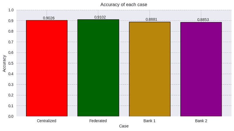
Let's plot the accuracies to each of the experiments:
predictions = [preds_cent, preds_fed, preds_bank_1, preds_bank_2]
titles = ["Centralized", "Federated", "Bank 1", "Bank 2"]
colors = ["red", "darkgreen", "darkgoldenrod", "darkmagenta"]
acc = [round(acc_cent,4), round(acc_fed,4), round(acc_bank_1,4) , round(acc_bank_2,4)]

s_plot_all_metric(acc, "Accuracy", titles, colors)
We can not obtain a conclusion by just studying this metric, since the dataset is really unbalanced. The model may be classifying almost all the classes as the predominant one. For that reason, the accuracy is almost 0.9 from all the cases.
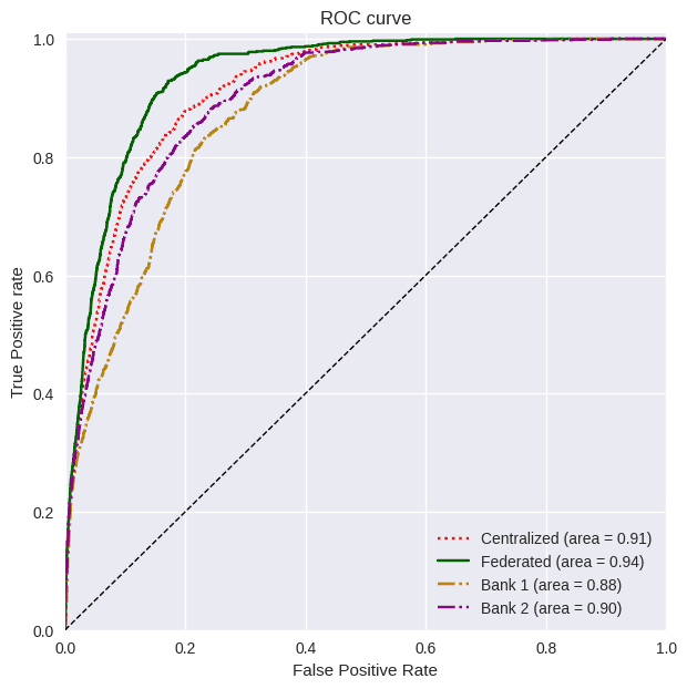
1-sum(test_labels==1)/sum(test_labels==0)0.87057856So if our model classifies all the label as the majority class (in this case, the class corresponding to the label 0) the accuracy would be that value. This means that the accuracy can not be trusted to make a decision about which model is better. Let's check the ROC curve:
linestyle = [":","-", "-.", "-."]

s_plot_all_roc_curves(test_labels, predictions, titles, colors, linestyle)
The ROC curve graph can not let us decide which classifier is having a better performance, since the AUC are very similar.
4.3) F1-Score
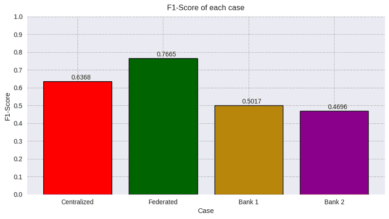
When the dataset is unbalanced, is better to study other kind of metrics such as F1-Score, that takes into account the precision and the recall. This way we will have a better judgement about which classifier has a better performance.
f1_scores = [round(f1_cent,4), round(f1_fed,4), round(f1_bank_1,4), round(f1_bank_2,4)]

s_plot_all_metric(f1_scores, "F1-Score", titles, colors)
This graphs is really interesting since it tells us that the local cases can not predict well enough. The centralized and federated case have a much better performance (26.92% and 52.78% repectively with the first Bank and 35.6% and 63.22% respectively with the second Bank). So it is clear that working with more data will improve the predictions. In this case, it looks like the federated case outperforms the centralized case. Theoretically, this can not happen, but we will discuss it in the conclusions.
5) Conclusion
This notebook is run with a seed of 987. To stablish a fair judgement about what is happening in this problem, we are going to run this experiment 10 different times. Then, we will obtain the mean and the standard deviation to observe the behaviour of the different cases:
- Accuracy
| Seed | Centralized | Federated | Bank 1 | Bank 2 |
|---|---|---|---|---|
| 25 | 0.893 | 0.9091 | 0.8846 | 0.8856 |
| 250 | 0.8914 | 0.9141 | 0.8959 | 0.8979 |
| 565 | 0.9013 | 0.909 | 0.8866 | 0.8866 |
| 70 | 0.9002 | 0.9142 | 0.8957 | 0.8905 |
| 5 | 0.9014 | 0.9149 | 0.8892 | 0.8890 |
| 1234 | 0.8865 | 0.9090 | 0.8863 | 0.8865 |
| 123 | 0.9027 | 0.9121 | 0.8885 | 0.8865 |
| 567 | 0.8911 | 0.9126 | 0.8911 | 0.8885 |
| 101 | 0.9000 | 0.9105 | 0.8850 | 0.8860 |
| 987 | 0.9026 | 0.9101 | 0.8878 | 0.8852 |
| Centralized | Federated | Bank 1 | Bank 2 | |
|---|---|---|---|---|
| Mean | 0.8970 | 0.9115 | 0.8891 | 0.8889 |
| Std | 0.0059 | 0.0023 | 0.0040 | 0.0041 |
The mean tells us that, in general. The standard deviation is very similar for all the cases in the accuracy, so no useful conclusion can be extracted with this information. Let's study that value in F1-Score:
- F1-Score
| Seed | Centralized | Federated | Bank 1 | Bank 2 |
|---|---|---|---|---|
| 25 | 0.559 | 0.7560 | 0.4694 | 0.4830 |
| 250 | 0.4713 | 0.7635 | 0.5189 | 0.5535 |
| 565 | 0.6354 | 0.7451 | 0.4699 | 0.4699 |
| 70 | 0.587 | 0.7657 | 0.5611 | 0.5088 |
| 5 | 0.6216 | 0.7697 | 0.4875 | 0.4717 |
| 1234 | 0.4699 | 0.7406 | 0.4698 | 0.4699 |
| 123 | 0.6363 | 0.7632 | 0.4704 | 0.4704 |
| 567 | 0.4712 | 0.7591 | 0.4712 | 0.4999 |
| 101 | 0.644 | 0.7601 | 0.4695 | 0.4832 |
| 987 | 0.6368 | 0.7664 | 0.4997 | 0.4698 |
| Centralized | Federated | Bank 1 | Bank 2 | |
|---|---|---|---|---|
| Mean | 0.5732 | 0.7589 | 0.4887 | 0.4879 |
| Std | 0.0754 | 0.0094 | 0.0305 | 0.0268 |
From this table we can observe that the deviation of the federated experiment is almost 8 times less than the centralized experiment. This tells us a really interesting insight: there will be cases, where a federated experiment is more robust than a centralized experiment. The centralized experiment is highly dependent on the initialization parameters, while in a federated experiment, this initialization is regularized due to the aggregation. In other words, the initialization of the weights has an important role in the way that a classifier makes its predictions. FedAvg softens this importance since it does a mean of the weights. This may be leading the problem to scape from a local minimum and converge to another minimum.